Data Structures
Notes on Data Structures. I also have notes on algorithms and general problem solving.
Heaps
A priority queue is an abstract data type that allows adding elements and retrieving the smallest or largest element. Priority queues are useful for an unbounded sequence for which we want to retrieve the $M$ smallest elements at any given moment.
The data structure commonly used to back a priority queue is an array embedding the contents of a complete binary tree in level-order that maintains two invariants:
- the parent of
$k$is$\left\lfloor (k - 1)/2 \right\rfloor$ - the children of
$k$are at$2k + 1$and$2k + 2$
Heap Insertion
| Case | Growth |
|---|---|
| Worst | $O(\log{n})$ |
Swimming in a heap is when a node is checked to ensure the invariant that every node is smaller than its parent. If a node’s value becomes larger than its parent, the node is swapped with its parent and the process is repeated at the new parent until the tree root is reached. This can be characterized as a new, larger node having to swim up the tree to its proper place.
To insert into the heap:
- add element to the end of the array
- increment heap size
- swim up the heap to restore heap order
private void swim(Comparable[] seq, int target) {
  // go up tree as long as the parent `target / 2` is
  // smaller than the child
  while (target >= 1 && seq[(target - 1) / 2] < seq[target]) {
    // swap parent and child
    swap(seq[(target - 1) / 2], seq[target]);

    // position is now that of previous parent
    target = (target - 1) / 2;
  }
}
Heap Removal
| Case | Growth |
|---|---|
| Worst | $O(\log{n})$ |
From a different perspective, if a node’s key becomes smaller than one or both of its children, the heap-order invariant will also be violated, because it conversely means that one or more of its children are larger than the parent. In this case, the node is simply swapped with the larger of its two children, a process known as sinking. This process is repeated for the new child all the way down the tree until the invariant holds.
To remove the maximum from the heap:
- take the largest item off of the top
- put the item from the end of the heap at the top
- decrement heap size
- sink down the heap to restore heap order
template <typename T>
void Sink(std::vector<T> &vec, int target) {
  using std::swap;

  while ((2 * target) + 1 < N) {
    // identify child of target
    int child = (2 * target) + 1;

    // choose right child if left child is smaller than right
    if (child < (N - 1) && vec[child] < vec[child + 1]) child++;

    // if the invariant holds, break
    if (vec[target] >= vec[child]) break;

    // otherwise swap with the larger child
    swap(vec[target], vec[child]);

    // position is now that of previously-larger child's
    target = child
  }
}
Heap Sort
| Case | Growth |
|---|---|
| Worst | $O(n\log{n})$ |
Heap sort is a sorting algorithm facilitated by a priority queue which performs well when backed by a binary heap. Heap sort more or less amounts to:
- feeding the sequence into a priority queue
- extracting the sequence out of the priority queue
However, there are certain details involved to make it operate faster. Usually these operations are performed in place to avoid using extra space.
First, the sequence has to be put into heap order, which is accomplished by walking up the tree (bottom-up) and sinking every root node with more than one child. The starting point for this is always $(N - 1) / 2$, which is the last node with two children. It’s important to note that “sinking a node” doesn’t mean that the node will definitively be swapped.
Assuming a maximum-oriented priority queue, the sorting is then accomplished by:
- swap the maximum with the last item in the heap
- decrease logical heap size
- sink the new root to ensure or repair heap order
- repeat 1-3 until the priority queue becomes empty
Note that the notion of a logical heap size is important, as the sorted sequence is increasingly added to the end of the same array that backs the heap, so it’s necessary to make a distinction between the two regions of the array, to prevent the heap sink or swim operations from corrupting the sorted region. This is accomplished in this code by using a hypothetical sink method that takes an upper bound parameter, which corresponds to the end of the heap region, i.e. the logical heap size.
template <typename T>
void Sort(std::vector<T> &vec) {
  using std::swap;

  const int N = vec.size();

  const int kLastElement = N - 1;
  const int kParentOfLastElement = (kLastElement - 1) / 2;

  // Arrange array into heap-order, starting from the last
  // node with two children and climbing up from there.
  for (int k = kParentOfLastElement; k >= 0; k--)
    sink(vec, k, N);

  // Move max to end of sorted region, which is to the right of
  // the unsorted region. Then sink the root node to ensure
  // heap order is preserved, but don't sink past the end of the
  // unsorted region, as that would corrupt the sorted region.
  while (N > 0) {
    swap(vec[0], vec[N--]);
    sink(vec, 0, N);
  }
}
Binary Search Trees
| Case | Growth |
|---|---|
| Worst | $O(n)$ |
This is the classical data structure consisting of a binary tree where each node has two children. The sub-tree to the left of each node consists of elements smaller than the node and the sub-tree to the right of each node consists of elements greater than the node.
The performance of BSTs greatly depends on the shape of the tree, which is a result of the distribution and order of the elements that are input.
The rank operation counts how many keys are less than or equal to the given value.
The predecessor of any node can be obtained easily if it has a left child, in which case the predecessor of the node is the maximum of the subtree rooted at the left child. If there is no left child, the predecessor is the first ancestor larger than the node (in other words, the first parent found for which the child is the right child). The successor can be found similarly, flipping left⟷right and maximum⟷minimum.
BST Structure
A perfect binary tree is one where every level has the maximum number of nodes.
The depth of a tree node is the number of edges from the root to the node, i.e. the level - 1, so the depth of the root node is 0. The level of a node in a tree is its depth + 1. The difference between levels and depth is that levels are the visual levels whereas depth is the number of edges from the root to the node.
The height of a tree node is the number of edges on the longest path from the node to a leaf. The height of an entire tree is the height of its root, i.e. the depth of the deepest node.
The number of levels in a binary tree with $n$ nodes is $\log_2 n$.
In a perfect binary tree, the number of nodes at depth $d$ is $2^d$.
In a perfect binary tree with $L$ levels, the total number of nodes is $2^L - 1$. So if there are 3 levels, $2^3 - 1 = 7$ total nodes.
BST Traversal
There are three main forms of traversing a BST. The order refers to the order in which the current node $C$ is visited, that is, the time at which $C$ is visited is the only thing that varies, so $L$ is always visited before $R$.
| Traversal | Order |
|---|---|
| pre-order | $C \to L \to R$ |
| in-order | $L \to C \to R$ |
| post-order | $L \to R \to C$ |
Morris Traversal
It’s possible to perform an in-order traversal of a BST without using a stack or recursion by performing a Morris traversal. In essence, this traversal transforms the tree during the traversal so that the entire right branch of the BST forms the in-order traversal. The BST is returned to its original structure as the traversal takes place.
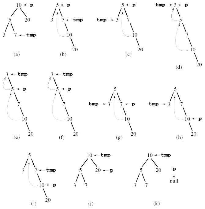
-
if left is
null -
visit
current -
go right
-
else:
-
set
temptocurrent’s left -
go right of
tempuntil its right isnullorcurrentThis finds the maximum of
current’s left, i.e. the in-order predecessor ofcurrent, or it finds the node whose right iscurrent. -
if
temp’s right isnull:This is the in-order predecessor of
current. Transform the tree so thattempleads tocurrentand is therefore in-order.- set
temp’s right tocurrent - go left of
current
This “rewinds” back to the last known minimum.
- set
-
if
temp’s right iscurrentThis is a node that was previously transformed to be in-order by making its right be
current. Repair transformation.- visit
current - unset
temp’s right (previouslycurrent) - go right of
current
- visit
-
while (current != null) {
    if (current.left == null) {
        visit(current);
        current = current.right;
    } else {
        temp = current.left;

        while (temp.right != null && temp.right != current) {
            temp = temp.right;
        }

        if (temp.right == null) {
            temp.right = current;
            current = current.left;
        } else {
            temp.right = null;
            visit(current);
            current = current.right;
        }
    }
}
BST Deletion
Most operations such as insertion and lookup are very straightforward. Deletion is somewhat more involved.
To delete node $k$:
$k$has no children: remove it$k$has just one child: swap it with child and delete it$k$has two children:- compute
$k$’s predecessor$l$, i.e. maximum of left subtree - swap
$k$and$l$ - delete
$k$ - now
$k$has no right child, recurse starting at 1
- compute
The transplant operation can be handled by simply associating the parent with the new child and vice versa:
void replace_node(tree *t, node *u, node *v) {
  if (u->p == t->nil)
    t->root = v;
  else if (u == u->p->left)
    u->p->left = v;
  else
    u->p->right = v;

  // ignore this check in red-black trees
  if (v != NULL)
    v->p = u->p;
}
BST Select
The BST can be augmented so that each node contains the count of notes rooted at it, including itself. Then the count can be computed for node $x$ base by adding the count of left child $y$ and right child $z$ plus one for $x$:
It’s important to keep this augmented information up-to-date with the operations on the tree, such as insertion or deletion, by traversing up the parents from the affected node to increment or decrement their counts.
Selection of the $i^\text{th}$ order statistic can be found easily by guiding the traversal of the tree with the augmented size information.
- the node in question is itself the ith order statistic, because
$a = i - 1$ - the
$i^\text{th}$order is somewhere in the left subtree, recurse - the
$i^\text{th}$order is somewhere in the right subtree, recurse. Since the right subtree only knows about itself, shift$i$to discard the left subtree and the root node.
T Select(node, int i) {
  int left_size = node->left ? size(node->left) : 0;

  // The current node is itself the ith order statistic
  if (left_size == i - 1) {
    return node->value;
  }

  // The ith order statistic is in the left subtree
  if (left_size >= i) {
    return Select(node->left, i);
  }

  // The ith order statistic is in the right subtree.
  // The right subtree only knows about itself, so shift the ith order
  // appropriately.
  if (left_size < i - 1) {
    return Select(node->right, i - left_size - 1);
  }
}
Augmented BST as Interval Tree
An interval search tree stores ranges and provides operations for searching for overlaps of a given range within the tree. A binary search tree can be augmented into an interval search tree. The lower bound of a range is used as the node key. Each node also stores the maximum upper bound of its children, similar to the rank.
For searching, the input interval is checked to see if it overlaps with the current node. If not, and the left node is null, search proceeds on the right child. If the left node’s max upper bound is less than the input interval’s lower bound, search proceeds on the right node. Otherwise search proceeds on the left node.
- if input interval
$[l, r]$overlaps current node, return - if left node is
nullor left’s max upper <$l$: go right
else: go left
Node current = root;

while (current != null) {
  if (current.interval.overlaps(lo, hi)) return current.interval;
  else if (current.left == null)         current = current.right;
  else if (current.left.max < lo)        current = current.right;
  else                                   current = current.left;
}

return null;
2-3 Search Trees
While 2-3 search tree can be implemented, they’re mainly used to help understand the implementation of Red-Black Trees, which have better performance.
A 2-3 tree is either empty or:
- 2-node: one key and two links
- left for keys smaller than the left key
- right for keys larger than the right key
- 3-node: two keys and three links
- left for keys smaller than the left key
- middle for keys between the node’s keys
- right for keys larger than the right key
2-3 Tree Searching
Searching follows simply from the structure of the tree.
- search hit if the key is in the node
- if not, recurse into the appropriate link
- search miss if a null link is reached
2-3 Tree Insertion
Insertion needs to take into consideration the fact that the tree must remain balanced after the operation. The general procedure is that the key is searched for until a node with a null link is reached at the bottom of the tree.
- single 2-node
- replace the 2-node with a 3-node containing the new key
- single 3-node
- create two 2-nodes out of each of the two keys
- replace the 3-node with a 2-node consisting of the new key
- set the 2-node’s links to the two new 2-nodes
- 3-node with 2-node parent (slight variation of above)
- create two 2-nodes out of each of the two keys
- move the new key into the parent 2-node to make it a 3-node
- set the middle link to the 3-node’s left key and right link to the right key
- 3-node with 3-node parent
- propagate the above operation until the root or a 2-node is encountered
- if the root is encountered, split it as in the case of a single 3-node
Perfect balance is preserved because tree height increase occurs at the root, and additions at the bottom of the tree are performed in the form of splitting existing nodes such that the height remains the same.
The problem with implementing a direct representation of 2-3 trees is that there are many cases to handle and nodes have to be converted between various types. These operations can incur overhead that nullifies or even makes worse the performance of 2-3 trees compared to regular BSTs.
Red-Black Trees
| Case | Growth |
|---|---|
| Worst | $O(2 \log {n})$ |
Red-Black trees are trees that guarantee near-perfect balance by maintaining 5 invariants:
- a node is either red or black
- root is black
- all leaves—represented as nil—are black
- both children of every red node are black, i.e. there must not be more than one red node in a row in any vertical path
- every path from a given node to any of its descendant leaves contains the same number of black nodes
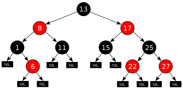
These properties allow red-black trees to be nearly balanced in even the worst case, allowing them more performance than regular BSTs. A very neat implementation is available here.
Red-Black Tree Insertion
The inserted node is attached in the same manner as for BSTs, except that every node is painted red on insertion. However, the inserted node has the possibility of violating any one of the 5 invariants, in which case the situation must be remedied. The following code representing the different cases that must be remedied are split into corresponding individual functions for didactic purposes.
There are three main scenarios that may arise from adding a node:
- first node added creates a red root, violating property 2 (root is black)
- node is added as child of black node, operation completes successfully
- consecutive red nodes, violating properties 4 (both children of red nodes are black) and 5 (equal number of black nodes per path)
Note that scenarios 1 and 3 violate the properties of red-black trees.
First, the inserted node may be the only node in the tree, making it the root. Since all nodes are inserted as red, it should be repainted black to satisfy property 2 (root is black):
void insert_case1(node *n) {
  if (n->parent == NULL)
    n->color = BLACK;
  else
    insert_case2(n);
}
Second, if the parent of the inserted node is black, the insertion is complete because it is not possible for that to have violated any of the properties:
void insert_case2(node *n) {
  if (n->parent->color == BLACK)
    return;
  else
    insert_case3(n);
}
Third, it is possible that the inserted node creates two consecutive red nodes, violating property 5 (equal number of black nodes per path). For this, there are three different scenarios:
- parent and uncle are both red
- direction in which new node and parent lean differ
- new node and parent lean in the same direction
First, if the parent and its uncle are red, flip their colors and make the grandparent red instead. This allows the newly added red node to satisfy all properties, since its parent is black. However, making the grandparent red may possibly violate properties 2 (root is black) and 4 (both children of red nodes are black), so recurse the enforcement algorithm on the grandparent starting from case 1:

void insert_case3a(node *n) {
  node *u = uncle(n), *g;

  if (u != NULL && u->color == RED) {
    n->parent->color = BLACK;
    u->color = BLACK;

    g = grandparent(n);
    g->color = RED;

    insert_case1(g);
  } else
    insert_case4(n);
}
Second, the new node could be added diagonal to a red parent node, meaning for example the parent node being red and the left child of its parent and the new node could be red (as always) and the right child of its parent.
This is ultimately resolved by two rotations, but the first rotation is made to get the new node leaning in the same direction as its parent. This is accomplished by rotating the new node in the direction of the parent’s direction from its parent. In the above example, the new node is its parent’s right child and the parent is the grandparent’s left child, so the new node is rotated left.
There are still consecutive red nodes after this rotation, albeit leaning in the same direction. This makes it simple for case 3c to handle, provided it is applied to the ex-parent, i.e. the now-bottom node, since case 3c operates in a more general sense from the perspective of the grandchild.

void insert_case3b(node *n) {
  node *g = grandparent(n);

  if (n == n->parent->right && n->parent == g->left) {
    rotate_left(n->parent);
    n = n->left;
  } else if (n == n->parent->left && n->parent == g->right) {
    rotate_right(n->parent);
    n = n->right;
  }

  insert_case5(n);
}
Third, the new node could be added below a red parent node and leaning in the same direction. For example, the new node is the left child of its parent and its parent is the left child of its parent (grandparent of the new node) as well.
This is resolved by rotating the grandparent in the direction opposite to the direction in which the consecutive red links lean. This has the effect of making the parent be the new root of the subtree previously rooted by the grandparent.
The grandparent was known to be black, since the red parent could not have been a child of it otherwise. Knowing this, the parent—now the root—switches colors with the grandparent, such that the subtree now consists of the black root and two red children.

void insert_case3c(node *n) {
  node *g = grandparent(n);

  n->parent->color = BLACK;
  g->color = RED;

  if (n == n->parent->left)
    rotate_right(g);
  else
    rotate_left(g);
}
Red-Black Tree Deletion
Deletion is handled similar to deletion in BSTs, but is a lot more complicated because the tree has to be re-balanced if removing a node from the tree causes it to become unbalanced.
Every resource I looked at—books, sites, university slides—simply hand-waived the deletion process presumably due to its complexity. The one place that managed to somewhat explain it well was the classic CLRS book, but its implementation consisted of a big, difficult-to-follow while-loop. Instead I decided to go with wikipedia’s long and dense explanation of its relatively simple implementation which even the Linux kernel uses.
First, if the node to be deleted has two children then it is replaced by its successor. The successor then has to be deleted, and by definition the successor will have at most one non-leaf child, otherwise it would not be the minimum in that subtree and the left child would have been followed.
void delete(node *m, void *key) {
  if (node == NULL) return;

  if      (*key < m->key) delete(m->left,  key);
  else if (*key > m->key) delete(m->right, key);
  else {
    if (m->left != NULL && m->right != NULL) {
      // replace with successor
      node *c = minimum_node(m->right);
      m->key = c->key;
      delete(c, c->key);
Second, if the node to be deleted has one child, simply replace the successor with its child.
    } else if (m->left != NULL || m->right != NULL) {
      // replace with child, delete child
      delete_one_child(m);
Third, if the node to be deleted has no children, then it is possible to simply delete it.
    } else {
      // no children, just delete
      free(m);
    }
  }
}
Red-Black Tree Balance
If the node is replaced with a successor, that successor is essentially removed from its original location, thereby possibly causing tree unbalanced. For this reason, the original successor node is removed using delete_one_child which re-balances the tree if necessary.
- node
$M$: successor to the node to be deleted - node
$C$: child of$M$, prioritized to be a non-leaf child if possible - node
$N$: child$C$in its new position - node
$P$:$N$’s parent - node
$S$:$N$’s sibling - nodes
$S_{L}$ and $S_{R}$:$S$’s left and right child respectively
First, if $M$ is red, then simply replace it with its child $C$ which must be black by property 4 (both children of red nodes are black). Any paths that passed through the deleted node will simply pass through one fewer red node, maintaining balance:
void delete_one_child(node *n) {
  node *child = is_leaf(n->right) ? n->left : n->right;

  replace_node(n, child);
Second, if $M$ is black and $C$ is red, paint $C$ black and put it in $M$’s place. This preserves the same amount of black nodes along that path:
  if (n->color == BLACK)
    if (child->color == RED)
      child->color = BLACK;
Third, the most complex case is when both $M$ and $C$ are black. Replacing one with the other effectively removes one black node along that path, unbalancing the tree. Begin by replacing $M$ with its child $C$, then proceed to the first re-balancing case:
    else
      delete_case1(child);

  free(n);
}
When both $M$ and $C$ are black nodes, four situations [^rbtree_case_merge] can arise that require re-balancing, unless $C$’s new position $N$ is the new root. If $C$ becomes the root it simply means that a black node was removed from all paths, effectively decreasing the black-height of every path by one and the tree therefore requires no re-balancing.
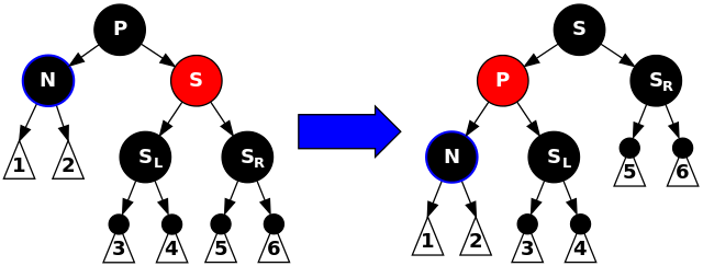
First: $N$’s sibling $S$ is red. In this case, reverse the colors of $P$ and $S$ and rotate $P$ left. Although all paths still have the same black-height, $N$’s sibling $S$ is now black and its parent $P$ is red, allowing fall-through to case 4, 5, or 6:
void delete_case1(node *n) {
  if (n->parent == NULL) return;

  node *s = sibling(n);

  if (s->color == RED) {
    n->parent->color = RED;
    s->color = BLACK;

    if (n == n->parent->left)
      rotate_left(n->parent);
    else
      rotate_right(n->parent);
  }

  delete_case2(n);
}
Second: $P$, $S$, and $S$’s children are all black. Repaint $S$ red so that all paths passing through $S$ have the same black-height as those that go through $N$.
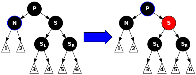
If $P$ is red, then the tree is violating property 4 (both children of red nodes are black), fix it by simply painting $P$ black.
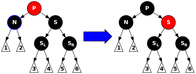
Otherwise, if $P$ was already black, however, then after the painting of $S$ to red, $P$ now has effectively lost one level from its black-height, so case 1 should be applied to $P$:
void delete_case2(node *n) {
  node *s = sibling(n);

  if (s->color == BLACK &&
      s->left->color == BLACK &&
      s->right->color == BLACK) {
    s->color = RED;

    if (n->parent->color == RED)
      n->parent->color = BLACK
    else
      delete_case1(n->parent);
  } else
    delete_case3(n);
}
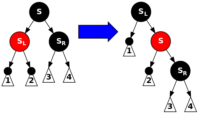
Third: $S$ is black, $S_{L}$ is red, $S_{R}$ is black, $N$ is left child of its $P$. Rotate $S$ right, then exchange colors of $S$ and its new parent. This case just prepares the tree for falling into case 6, since $N$ now has a black sibling—$S_{L}$—whose right child is red.
void delete_case3(node *n) {
  node *s = sibling(n);

  if (s->color == BLACK) {
    if (n == n->parent->left &&
        s->right->color == BLACK &&
        s->left->color == RED) {
      s->color = RED;
      s->left->color = BLACK;
      rotate_right(s);
    } else if (/* symmetric to above */) { }
  }

  delete_case4(n);
}
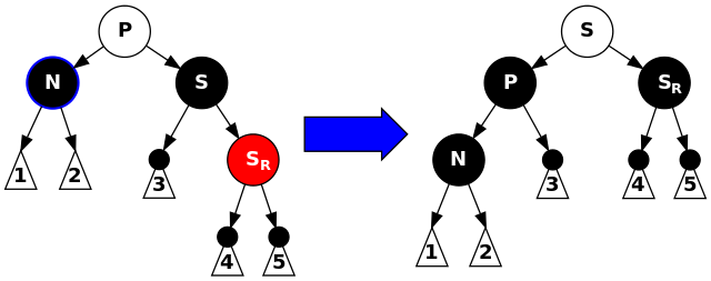
Fourth: $S$ is black, $S_{R}$ is red, $N$ is left child of its $P$. Rotate $P$ left, exchange colors of $P$ and $S$, and make $S_{R}$ black.
This unbalances the tree by increasing black-height of paths through $N$ by one because either $P$ became black or it was black and $S$ became a black grandparent.
void delete_case4(node *n) {
  node *s = sibling(n);

  s->color = n->parent->color;
  n->parent->color = BLACK;

  if (n == n->parent->left) {
    s->right->color = BLACK;
    rotate_left(n->parent);
  } else {
    s->left->color = BLACK;
    rotate_right(n->parent);
  }
}
Interval Trees
Interval trees are useful for efficiently finding all intervals that overlap with any given interval or point.
To construct the tree, the median of the entire range of all of the set of ranges is found. Those ranges in the set that are intersected by the median are stored in the current node. Ranges that fall completely to the left of the median are stored in the left child node, and vice versa with the right node.
At any given node representing the set of ranges intersected by the median at that node, two sorted lists are maintained: one containing all beginning points and the other containing all end points.
Hash Tables
Hash tables consist of an array coupled with a hash function—such as MurmurHash or CityHash—and a collision resolution scheme, both of which help map the key to an index within the array.
Hash Tables can be used for de-duplication, as well as keeping track of what states have already been seen in search algorithms, especially for those applications where it’s not feasible to store all of the nodes.
In the 2-SUM problem, given an unsorted array of $n$ integers and a target sum $t$, we need to find if there is a pair of integers that sum to $t$.
The brute-force approach is to check all possible pairs in $O(n^2)$ to see if they add up to the target $t$.
Alternatively, we can sort the array in $O(n \log n)$ and scan through the array, for each element $x$ determine the required summand $r = t - x$, then look for $r$ in the array using binary search $O(n \log n)$. If $r$ is found, then there’s a match, i.e. $x + r = t$.
This can be improved further by using a hash table. Put each element of the array into a hash table, then for each element $x$ in the array compute the required summand $r = t - x$ and check if $r$ is present in the hash table. If so, then there’s a match.
Hash Functions
Hash functions need to be consistent, efficient, and should uniformly distribute the set of keys.
A popular and simple hashing function is modular hashing of the form:
where $k$ is the key and $M$ is the array size, used to avoid integer overflow, usually chosen to be prime. Multiple pieces of data can be combined into one hash by doing:
where $R$ is a prime number such as a 31, $H$ is the hash as constructed so far (initially set to some prime number) and $D$ is the new piece of data.
For example, given a three properties—day, month, and year—the following hash computation could be used:
int hash = 0;
int hash = (hash * R + day  ) % M;
int hash = (hash * R + month) % M;
int hash = (hash * R + year ) % M;

// or
int hash = (((((0 * R + day) % M) * R + month) % M) * R + year) % M;
Or to hash a given string:
int hash = 0;

for (int i = 0; i < s.length(); i++)
  hash = (R * hash + s.charAt(i)) % M;
A simpler hashing scheme that doesn’t account for integer overflow is:
So for example, given a day, month, and year:
int hash = R + day;
int hash = hash * R + month;
int hash = hash * R + year;

int hash = ((R + day) * R + month) * R + year;
Pathological Data Sets
It’s possible to craft a pathological data set that can cause a denial of service attack on a hash table.
One way to mitigate this is to use a cryptographic hash function, which also has pathological data sets but it’s less feasible to discover them.
Alternatively, design a family of hash functions and choose one randomly.
Load Factor
The load factor is defined by $\alpha = N/M$ where $\alpha$ is the percentage of table entries that are occupied, $N$ is the number of objects in the hash table, and $M$ is the number of buckets in the hash table.
Note that a load factor is still relevant in an open addressing scheme, in which case each bucket can only hold one value.
In linear probing, $\alpha$ can never be 1 because if the table becomes full, a search miss would go into an infinite loop. Instead, array resizing is performed to ensure that the load factor is between $\frac {1} {8}$ and $\frac {1} {2}$.
The average number of compares, or probes, in a linear-probing hash table of size $M$ and $N = \alpha M$ keys is:
Based on this, when $\alpha$ is about 0.5 there will be 1.5 compares for a search hit and 2.5 compares for a search miss on average. For this reason, $\alpha$ should be kept under 0.5 through the use of array resizing.
Separate Chaining
| Case | Growth |
|---|---|
| Worst | $O(\log {n})$ |
This collision resolution strategy involves storing a linked-list at every entry in the array. The intent is to choose the size of the array large enough so that the linked-lists are sufficiently short.
Separate chaining consists of a two-step process:
- hash the key to get the index to retrieve the list
- sequentially search the list for the key
A property of separate chaining is that the average length of the lists is always $N/M$ in a hash table with $M$ lists and $N$ keys.
Double Hashing
Double hashing is a form of open addressing in which two hash functions are used. If the first hash function incurs a collision, then the result of the second hash function serves as an offset at which to try insertion. For example, if $h_1(x) = 17$ caused a collision, and $h_2(x) = 23$, then it will try inserting at position $17 + 23 = 40$, then $40 + 23 = 63$, and so on.
Linear Probing
| Case | Growth |
|---|---|
| Worst | $O(c \log {n})$ |
Linear probing is a form of open addressing that relies on empty entries in the array for collision resolution. Linear probing simply consists of:
- hash the key to get the index
- the element at the index determines three outcomes:
- if it’s an empty position, insert the element
- if the position is not empty and the key is equal, replace the value
- if the key is not equal, try the next entry and repeat until it can be inserted
Linear Probing Deletion
The insert and retrieval operations retrieve the index and perform the same operation until the entry is null. This has the consequence that deleting a node cannot simply entail setting the entry to null, or it would prematurely stop the lookup of other keys.
As a result, after setting the entry to null, every key to the right of the removed key also has to be removed, i.e. set to null, and then re-inserted into the hash table using the regular insertion operation.
Sparse Vectors
An application of hash tables can be to implement sparse vectors for the purpose of performing matrix-vector multiplications. In certain situations, the row-vector from a matrix can have a very small amount of non-zero elements. If the matrix was stored in a naive array format it would amount to an immense waste of space and computation.
Instead, sparse vectors are vectors backed by hash tables where the keys correspond to the index of a given element and the value corresponds to that element’s value. This solution is used in Google’s PageRank algorithm.
Bloom Filters
Bloom filters are useful for remembering which values have been seen; they don’t store the actual values or keys, so they use very little space. There are no deletions.
Membership lookups can yield false-positives, but not false-negatives. So a bloom filter can answer if an element is possibly in the set or definitely not in the set.
For example, a bloom filter could be used to back a spell-checker. All correctly spelled words are inserted into the bloom filter, then a word can be checked for correct spelling by checking if it’s in the bloom filter. However, since there is a small possibility of a false-positive, it may incorrectly determine that the word is correctly spelled even if it’s not.
Bloom filters are often used in network routers for tasks such as keeping track of blocked IP addresses, the contents of a cache to avoid spurious lookups, and maintaining statistics to prevent denial of service attacks.
Bloom filters consist of a bitset, where each entry uses $\frac n {|S|}$ bits. The bloom filter has $k$ hash functions.
Insertion is accomplished by hashing the input with each of the $k$ hash functions and turning on the bit at that position, regardless of whether that bit was already on.
for (const auto &hash_function : hash_functions) {
  bits |= (1 << hash_function(x));
}
Lookup is accomplished by hashing the input with each hash function and checking if all of those positions is on.
for (const auto &hash_function : hash_functions) {
  if (!(bits & (1 << hash_function(x)))) {
    return false;
  }
}

return true;
Therefore the false-positives come about if other insertions set the same bits as those used by other elements.
Tries
Trie structures exploit string properties to provide much faster string search, with hits taking time proportional to the length of the key and where misses require examining only a few characters.
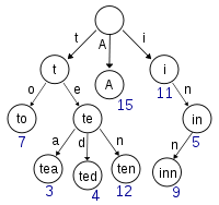
The structure of tries is comprised of a tree where every node has $R$ links where $R$ is the size of the alphabet. Every node also has an associated label corresponding to the character value consumed to reach the node. The root node has no such label as there is no link pointing to it. Every node also also has an associated value corresponding to the value associated with the key denoted by the path ending at the particular node.
A search hit occurs when the trie search arrives at the final node and that node’s value is not empty. A search hit occurs both if the final node’s value is empty or if the search terminated on a null link.
Value get(String key) {
  Node x = get(root, key, 0);
  if (x == null) return null;
  return x.val;
}

Node get(Node x, String key, int d) {
  if (x == null) return null;
  if (d == key.length()) return x;
  char c = key.charAt(d);
  return get(x.next[c], key, d + 1);
}
Trie insertion simply consists of searching for the key and setting the value. If the key does not already exist, then create nodes for every character not yet in the trie.
void put(String key, Value val) { root = put(root, key, val, 0); }

Node put(Node x, String key, Value val, int d) {
  if (x == null) x = new Node();
  if (d == key.length()) { x.val = val; return x; }
  char c = key.charAt(d);
  x.next[c] = put(x.next[c], key, val, d + 1);
  return x;
}
Tries also allow operations for collecting keys with a common prefix. This is accomplished by finding the node at the end of the prefix’ path and then recursively performing BFS on every node and enqueueing any node that has a non-empty value.
Queue<String> keysWithPrefix(String prefix) {
  Queue<String> q = new Queue<String>();
  collect(get(root, prefix, 0), prefix, q);
  return q;
}

void collect(Node x, String prefix, Queue<String> q) {
  if (x == null) return;
  if (x.val != null) q.enqueue(prefix);

  for (char c = 0; c < R; c++)
    collect(x.next[c], prefix + c, q);
}
This can also be modified to allow wildcard pattern matches, for example, keys that match fin. could include fine, find, etc.
Queue<String> keysWithPrefix(String pattern) {
  Queue<String> q = new Queue<String>();
  collect(root, "", pattern, q);
  return q;
}

void collect(Node x, String prefix, String pattern, Queue<String> q) {
  int d = pre.length();

  if (x == null) return;
  if (d == pattern.length() && x.val != null) q.enqueue(prefix);
  if (d == pattern.length()) return;

  char next = pattern.charAt(d);
  for (char c = 0; c < R; c++)
    if (next == '.' || next == c)
      collect(x.next[c], prefix + c, pattern, q);
}
Trie Deletion
Deletion is a straightforward process in tries, simply involving finding the node and emptying its value. If this operation makes the node’s parent’s children all be null, then the same operation must be run on the parent.
void delete(String key) { root = delete(root, key, 0); }

Node delete(Node x, String key, int d) {
  if (x == null) return null;
  if (d == key.length())
    x.val = null;
  else {
    char c = key.charAt(d);
    x.next[c] = delete(x.next[c], key, d + 1);
  }

  if (x.val != null) return x;

  for (char c = 0; c < R; c++)
    if (x.next[c] != null)
      return x;

  return null;
}
Ternary Search Trees
Ternary Search Trees (TSTs) seek to avoid the excessive space cost of regular R-way tries demonstrated above. TSTs are structured such that each node has only three links for characters less than, equal to, and greater than the node.
R-way tries can provide the fastest search, finishing the operation with a constant number of compares. However, space usage increases rapidly with larger alphabets TSTs are preferable, sacrificing a constant number of compares for a logarithmic number of compares.
Node get(Node x, String key, int d) {
  if (x == null) return null;
  char c = key.charAt(d);

  if      (c < x.c) return get(x.left,  key, d);
  else if (c > x.c) return get(x.right, key, d);
  else if (d < key.length() - 1)
                    return get(x.mid,   key, d);
  else return x;
}
Insertion is similar to insertion with tries except that only one of three links can be taken, instead of $R$ links.
void put(String key, Value val) { root = put(root, key, val, 0); }

Node put(Node x, String key, Value val, int d) {
  char c = key.charAt(d);

  if (x == null) { x = new Node(); x.c = c; }

  if      (c < x.c) x.left  = put(x.left,  key, val, d);
  else if (c > x.c) x.right = put(x.right, key, val, d);
  else if (d < key.length() - 1)
                    x.mid   = put(x.mid,   key, val, d + 1);
  else x.val = val;
  return x;
}
B-Trees
A B-Trees of order $M$ is a tree consisting of internal and external $k$-nodes each consisting of $k$ keys where $2 \leq k \leq M - 1$ at the root and $M/2 \leq k \leq M - 1$ at every other node. Internal nodes contain copies of keys, where every key is greater than or equal to its parent node’s associated key, but not greater than the parent node’s next largest key. External nodes are the leaves of the tree that associate keys with data. A sentinel key is created to be less than all other keys and is the first key in the root node.
B-Tree Insertion
To insert a key, the tree is recursively descended by following the link pertaining to the interval upon which the inserted key falls until an external node is reached. The tree is balanced on the way up the tree after the recursive call. If a node is full it is split into two $M/2$-nodes and attached to a parent 2-node (if at the root) or a $(k + 1)$-node where $k$ was the original size of the full node’s parent. Whenever a node is split, the smallest key in the new node (or both smallest keys from both nodes if at the root) is inserted into the parent node.
void add(Key key) {
  add(root, key);

  if (root.isFull()) {
    Page left = root;
    Page right = root.split();

    root = new Page();
    root.add(left);
    root.add(right);
  }
}

void add(Page h, Key key) {
  if (h.isExternal()) { h.add(key); return; }

  Page next = h.next(key);
  add(next, key);

  if (next.isFull())
    h.add(next.split());

  next.close();
}
Suffix Arrays
Suffix arrays are arrays of suffixes of a given text which help with procedures such as finding the longest repeated substring in some text.
class SuffixArray {
  private final String[] suffixes;
  private final int N;

  public SuffixArray(String s) {
    N = s.length();
    suffixes = new String[N];
    for (int i = 0; i < N; i++) suffixes[i] = s.substring(i);
    Array.sort(suffixes);
  }

  public int lcp(String s, String t) {
    int N = Math.min(s.length(), t.length());
    for (int i = 0; i < N; i++) if (s.charAt(i) != t.charAt(i)) return i;
    return N;
  }

  public int lcp(int i) { return lcp(suffixes[i], suffixes[i - 1]); }
  public int rank(String key) { /* binary search */ }
  public String select(int i) { return suffixes[i]; }
  public int index(int i) { return N - suffixes[i].length(); }
}
Using this suffix array class, the longest repeated substring can be found efficiently:
void main(String[] args) {
  String text = StdIn.readAll();
  int N = text.length();
  SuffixArray sa = new SuffixArray(text);
  String lrs = "";

  for (int i = 1; i < N; i++) {
    int length = sa.lcp(i);
    if (length > lrs.length())
      lrs = sa.select(i).substring(0, length);
  }

  StdOut.println(lrs);
}