Algorithms
What follows are some notes on algorithms I’ve been reviewing from Algorithms by Robert Sedgewick and Kevin Wayne, The Algorithm Design Manual by Steven S. Skiena, and other sources around the Internet 1 2 3. I wanted to write some notes on the material so that I could easily look back on it, but mainly so that I could be sure that I understand the material.
I also have notes on data structures and notes on general problem solving.
Analysis
The goal of asymptotic analysis is to suppress the constant factors and lower-order terms. This is because the constant factors are very system-dependent, such as how many cycles a certain operation may take between different pieces of hardware. The lower-order terms are also not as important because they are rendered irrelevant for very large inputs, where the higher-order terms dominate.
| Name | Complexity | Examples |
|---|---|---|
| Constant | $O(1)$ |
Adding two numbers |
| Logarithmic | $O(\log n)$ |
Branching |
| Linear | $O(n)$ |
Scanning the input |
| Linearithmic | $O(n \log n)$ |
Branching and scanning at each level |
| Quadratic | $O(n^2)$ |
Looking at all pairs of an input |
| Cubic | $O(n^3)$ |
Looking at all triples of an input |
| Exponential | $O(c^n)$ |
Looking at all subsets of an input |
| Factorial | $O(n!)$ |
Looking at all permutations/orderings of $n$ items |
Summations
The summation of a constant is simply the product of the constant and the range:
The sum of the first $n$ integers can be visualized as folding the range of values at the middle so that the first integer is paired with the last, or more generally: the $i^\text{th}$ paired with the $(n - i + 1)\text{th}$. Below, the bound of $n/2$ refers to the “folding at the middle,” then each pair is added. Note that the sum is quadratic.
The sum of a harmonic series is approximately equal to the logarithm of the bound.
Logarithms
The exponent of a logarithm operand can be extracted:
Bounds
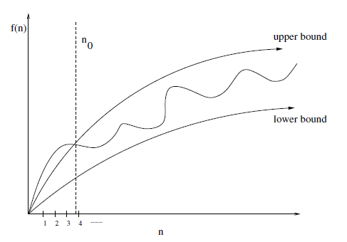
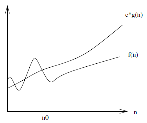
The upper-bound $f(n) = O(g(n))$ means that there exists some constant $c$ such that $f(n)$ is always $\le c \cdot g(n)$ for a large enough $n$, that is, for some offset $n_0$ such that $n \ge n_0$.
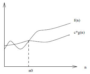
The lower-bound $f(n) = \Omega(g(n))$ is similar except that it is a lower-bound, so that there exists some constant $c$ such that $f(n)$ is always $\ge c \cdot g(n)$ for $n \ge n_0$.
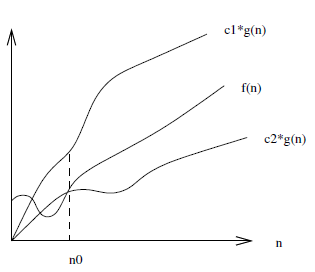
There is also $f(n) = \Theta(g(n))$ which means that $c_1 \cdot g(n)$ is an upper-bound and $c_2 \cdot g(n)$ is a lower-bound on $f(n)$ for $n \ge n_0$. This is a tighter bound on $f(n)$ than simply a lower or upper-bound alone would provide.
Constant factors are ignored since they can easily be beaten out by a different chosen value of $c$.
Dominance Relations
A faster-growing function $f(n)$ dominates a slower-growing one $g(n)$, i.e. $f \gg g$.
When analyzing an algorithm it is common to produce an expression of bounds which can easily be simplified by keeping in mind the principle of dominance relations.
Sum of Bounds
For example, if an algorithm first sorts its input and then prints each element, then that’s a sorting operation of $O(n \log n)$ followed by a linear printing operation of $O(n)$, essentially becoming $O(n \log n + n)$. However, the linearithmic term clearly dominates the linear term, so simplifying it to $O(n \log n)$ still leaves an accurate bound.
Product of Bounds
Constant factors are ignored since a different value of the constant $c$ can be chosen to compensate for any arbitrary constant factor.
However, the product of functions is important. For example, a linear scan of an array in $O(n)$ where for each element another linear scan of the array is made in $O(n)$ produces a product of $O(n \cdot n) = O(n^2)$.
Master Theorem
The master theorem provides a straightforward, “black-box” way of determining the running time of a recursive, divide-and-conquer algorithm. It’s stated as:
where:
$n$is the size of the problem$a$is the number of recursive calls per level$\frac n b$is the size of each subproblem$f\left(n^d\right)$is the work done outside of the recursive calls, e.g. the merge in mergesort
Then the run-time complexity of an algorithm can be determined based on the values of $a$, $b$, and $d$.
-
when
$a = b^d$, the complexity is$O\left(n^d \log n\right)$The same amount of work
$n^d$is being done at each level, of which there are$\log n$.
-
when
$a < b^d$, the complexity is$O\left(n^d\right)$Most of the work is done at the root, as if only at a single level.
-
when
$a > b^d$, the complexity is$O\left(n^{\log_b a}\right)$It’s equivalent to the number of leaves in the recursion tree, since most of the work is done at the bottom of the tree.
Essentially, the master theorem is a tug-of-war between:
$a$: the rate of subproblem proliferation$b^d$: the rate of work shrinkage per subproblem
Approximations
Oftentimes it’s useful to use approximations instead of exact values.
Stirling’s approximation:
Intractability
An intractable problem is one that has no efficient solution. It can be proved that a problem is intractable if a known intractable problem can be reduced to the given problem.
- change the problem formulation such that it still achieves the higher goal
- brute-force or dynamic programming: acceptable if instances or exponential parameter is small
- search: prune search-space via backtracking, branch-and-bound, hill-climbing
- heuristics: insight, common case analysis
- parallelization: solve subparts in parallel
- approximation: solution that is provably close to optimum
Sorting
The following algorithms are described with the assumption that the sequence is an array of contiguous memory and constant access time. This is noteworthy because it is important to recognize algorithms can have different speeds depending on the underlying data structure.
For example, selection sort backed by a priority queue or balanced binary tree can help to speed up the operation of finding the smallest element in the unsorted region. Instead of being linear, the operation would be $\log(n)$. Given that this is done at every element in the sequence, of which there are $N$, this means that selection sort backed by such a structure can be improved from $O(n^2)$ to $O(n\log(n))$ 4.
A sorting algorithm is known as stable if it maintains the same relative order of equal keys as it was before the sorting operation.
The best case complexity of comparison-based sorting is $O(n \log n)$. If the distribution of the data is known, sorting can be done much faster using counting or bucket sort, for example.
Many problems can be reduced to sorting.
Selection Sort
| Case | Growth |
|---|---|
| Any | $\Theta(n^2)$ |
This is a pretty naive algorithm that is mainly useful for didactic purposes.
Algorithm operation:
- go through entire sequence to find smallest element
- swap element with the left-most unsorted element
- repeat until the end of the sequence
This essentially splits the sequence into a left sorted region and a right unsorted region.
template<typename T>
void sort(std::vector<T> &sequence) {
  int size = sequence.size();

  for (int i = 0; i < size; i++) {
    int min = i;

    for (int j = i + 1; j < size; j++) {
      if (sequence[j] < sequence[min]) {
        min = j;
      }
    }

    swap(sequence[i], sequence[min]);
  }
}
Insertion Sort
| Case | Growth |
|---|---|
| Best | $\Theta(n)$ |
| Worst | $O(n^2)$ |
This is a stable algorithm that is still pretty straightforward but somewhat improves upon selection sort if the array is already sorted or if it’s nearly sorted.
It operates as follows:
- go through the entire sequence until an element is found which is smaller than the previous element
- swap the smaller element with the one on the left until the element to its left is no longer larger than itself
- repeat until the end of the sequence
The benefit of insertion sort is that if the sequence is already sorted then the algorithm operates in linear time. Similarly, if the sequence is nearly sorted, the algorithm will perform better than the worst case.
Performance Factors: order of the items
template<typename T>
void sort(std::vector<T> &sequence) {
  int size = sequence.size();

  for (int i = 0; i < size; i++) {
    for (int j = i; j > 0; j--) {
      if (sequence[j] < sequence[j - 1]) {
        swap(sequence[j], sequence[j - 1]);
      } else {
        break;
      }
    }
  }
}
Shell Sort
| Case | Growth |
|---|---|
| Worst | $O(n^{3/2})$ |
While insertion sort can be faster than selection sort, one problem with it is that the swap operations are done one at a time. This means that in the worst case, when sorting position 1 of the array, the smallest element could be at the very end of the array, meaning a total of $N - 1$ swaps where $N$ is the length of the array.
Shell sort aims to mitigate this by doing the following:
- pick a large number
$H$some constant factor less than the length of the sequence - consider every
$H^{th}$element in the sequence and apply insertion sort to those elements - now consider every
$(H + 1)^{th}$element and do the same - repeat incrementing
$H$until the end of the array is reached - repeat steps 2 - 4 but with
$H$reduced by some factor until the reduction reaches$1$ - ultimately do regular insertion sort, i.e.
$H = 1$
The value picked for $H$ and the factor which is used to reduce it form what is known as a gap sequence. The overall worst-case time complexity depends on the chosen gap sequence. A commonly chosen gap sequence with a worst-case time complexity of $O(n^{3/2})$ is:
This sequence begins at the largest increment less than $N/3$ and decreases to 1. This means that for a sequence of length $16$ the sequence is $13, 4, 1$.
The effect of shell sort is that it sorts elements that are $H$ elements apart with one swap instead of $H$. The granularity of the sorting operation increases as $H$ itself decreases such that every element is eventually sorted, but with the added benefit that as $H$ decreases, the distance of the longest-distance swap decreases.
template<typename T>
void sort(std::vector<T> &sequence) {
  int size = sequence.size();
  int h = 1;

  while (h < N/3) {
    h = 3 * h + 1;
  }

  while (h >= 1) {
    for (int i = h; i < size; i++) {
      for (int j = i; j >= h; j -= h) {
        if (sequence[j] < sequence[j - h]) {
          swap(seq[j], sequence[j - h]);
        } else {
          break;
        }
      }
    }

    h = h / 3;
  }
}
Merge Sort
| Case | Growth |
|---|---|
| Worst | $O(n\log{n})$ |
| Space | $O(n)$ |
This is a stable algorithm and the first algorithm that is linearithmic in complexity. The general idea is that the sequence is split into many pieces and then they’re all merged back together. The sorting occurs during the merging phase. The merging algorithm works such that the resultant merged piece is sorted.
The main drawback is that it has $O(n)$ space complexity because an auxiliary sequence has to be created to facilitate the merging process.
def merge(seq, aux, lo, mid, hi):
    for i in range(lo, hi):
        aux[i] = seq[i]

    left = lo
    right = mid
    i = lo

    while left < mid or right < hi:
        both = left < mid and right < hi

        if right == hi or (both and aux[left] < aux[right]):
            seq[i] = aux[left]
            left += 1

        else:
            seq[i] = aux[right]
            right += 1

        i += 1
The complexity is $O(n \log n)$ because the number of subproblems is doubling at each level (i.e. the two recursive calls), but the work to be done by those subproblems is halving. That is, for a given level $j$, the amount of work done is:
Given an input size of $n$, the number of levels in the recursion tree is $\log_2 n$, which means that at each of the $\log_2 n$ levels in the tree there is $n$ work being done, hence $n \log n$.
Top-Down
This is a recursive approach that works by splitting the array into two pieces until the pieces consist of pairs of elements. On each recurrence, the two pieces that were split for that recurrence are merged back.
def mergesort(seq):
    aux = seq[:]

    sort(seq, aux, 0, len(seq))

    return seq

def sort(seq, aux, lo, hi):
    if (hi - lo) <= 1: return

    mid = lo + ((hi - lo) // 2)

    sort(seq, aux, lo, mid)
    sort(seq, aux, mid, hi)

    merge(seq, aux, lo, mid, hi)
There are a couple of improvements that can be made to top-down merge sort:
- use insertion sort for small sub-arrays: create a cut-off, e.g. 15 elements, where the pieces are sorted with insertion sort instead of being broken down further
- test if sequence is already in order: skip the merging phase if
seq[mid] <= seq[mid + 1]
Bottom-Up
The other approach to merge sort is bottom-up, that is, starting with arrays consisting of one element and merging them together, then merging all of the arrays of size two, and so on until the entire array is merged.
- increments a counter
$SZ$in the series of powers of two until$SZ < N$ - merges every sub-array of length
$2SZ$
One advantage of bottom-up merge sort is that it can be modified to perform on linked-lists in place.
template<typename T>
void sort(std::vector<T> &sequence) {
  int size = sequence.size();
  aux = std::vector<T>(size);

  for (int sz = 1; sz < N; sz = sz + sz) {
    for (int lo = 0; lo < N - sz; lo += sz + sz) {
      merge(sequence, lo, lo + sz - 1, min(lo + sz + sz - 1, N - 1));
    }
  }
}
Quick Sort
| Case | Growth |
|---|---|
| Worst | $O(n^2)$ |
| Average | $O(n \log n)$ |
| Space | $O(\log n)$ |
QuickSort works by choosing an element in the array—the pivot—and partitioning the array such that all elements less than the pivot are moved to its left and all elements greater than the pivot are moved to its right. This has the effect that, at the end of this operation, the chosen element will be at its “sorted order position,” i.e. the position in which it would be if the entire array were already sorted.
Note that the elements are simply moved to the correct side of the pivot, but the order of neither side is defined, i.e. neither the left nor the right side are necessarily sorted after partitioning.
template<typename T>
void sort(std::vector<T> &sequence) {
  shuffle(sequence);

  sort(sequence, 0, sequence.size() - 1);
}

template<typename T>
void sort(std::vector<T> &sequence, int lo, int hi) {
  if (hi <= lo) {
    return;
  }

  int j = partition(sequence, lo, hi);

  sort(sequence, lo, j - 1);
  sort(sequence, j + 1, hi);
}
The partition algorithm is similar to merge in merge sort in that it is what actually does the sorting.
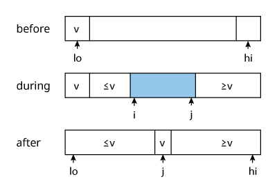
- choose a partition element separator
$v$ - scan through the array from
$i$to$j$in both directions- while
$i < v$doi++ - while
$j > v$doj-- - swap
$i$and$j$
- while
- repeat step 2 until the iterators
$i$and$j$cross - swap the partition element
$v$with the final position of the right-side iterator$j$
The sorting algorithm then recurses on the two partitions. Note that i is set to lo and not lo + 1 to ensure that the pivot at lo is skipped, since the first operation is ++i. However, j is set to hi + 1 to ensure that hi is not skipped, since it’s not the pivot.
template<typename T>
int partition(std::vector<T> &sequence, int lo, int hi) {
  T v = sequence[lo];
  int i = lo;
  int j = hi + 1;

  while (true) {
    while (sequence[++i] < v) {
      if (i == hi) {
        break;
      }
    }

    while (v < sequence[--j]) {
      if (j == lo) {
        break;
      }
    }

    if (i >= j) {
      break;
    }

    swap(sequence[i], sequence[j]);
  }

  swap(sequence[lo], sequence[j]);
  return j;
}
Quick Sort Improvements
-
use insertion sort for small sub-arrays: Adding a cutoff size for which to apply insertion sort to small sub-arrays can improve the performance of the algorithm.
Instead of:
if (hi <= lo) return;use:
if (hi <= lo + M) { insertionSort(sequence, lo, hi); return; }where
Mis the cutoff. Recommended sizes are between 5 and 15. -
median-of-three partitioning: Choose a sample of size 3 from the sequence and choose the middle element as the partitioning element.
Three-way Partitioning
| Case | Growth |
|---|---|
| Best | $O(n)$ |
| Worst | $O(n\log{n})$ |
| Space | $O(\log{n})$ |
One problem with quick sort as it is implemented above is that items with keys equal to that of the partition item are swapped anyways, unnecessarily. Three-way partitioning aims to resolve this by partitioning into three separate sub-arrays, the middle of which corresponds to those items with keys equal to the partition point. E. W. Dijkstra popularized this as the Dutch National Flag problem.
Performance Factors: distribution of the keys
- perform a 3-way comparison between element
$i$and$v$$seq[i] < v$: swap$lt$and$i$andlt++andi++$seq[i] > v$: swap$i$and$gt$andgt--$seq[i] = v$:i++
- repeat step 1 until
$i$and$gt$cross, i.e. while$i \leq gt$ - recurse on the left and right segments
Quick sort performs a lot better than merge sort in sequences that have duplicate keys. Its time is reduced from linearithmic to linear for sequences with large numbers of duplicate keys.
template<typename T>
void sort(std::vector<T> &sequence, int lo, int hi) {
  if (hi <= lo) {
    return;
  }

  int lt = lo;
  int i = lo + 1;
  int gt = hi;

  T v = sequence[lo];

  while (i <= gt) {
    int cmp = (sequence[i] > sequence[v]) - (sequence[i] < sequence[v]);

    if (cmp < 0) {
      swap(sequence[lt++], sequence[i++]);
    } else if (cmp > 0) {
      swap(sequence[i], sequence[gt--]);
    } else {
      i++;
    }
  }

  sort(sequence, lo, lt - 1);
  sort(sequence, gt + 1, hi);
}
Graphs
A graph is a set of vertices and a collection of edges that each connect a pair of vertices. This definition allows for self-loops (edges that connect a vertex to itself) and parallel edges (multiple edges connecting the same vertex pair).
Graphs with parallel edges are sometimes known as multigraphs, whereas graphs with no parallel edges or self-loops are simple graphs.
Two vertices connected by an edge are adjacent, and the edge is incident to both vertices. A vertex’ degree is the number of edges connected to it. A subgraph is a sub-set of edges and associated vertices that still constitutes a graph.
Paths in graphs are sequences of vertices connected by edges. Simple paths have no repeated vertices. A path forms a cycle if it has at least one edge whose first and last vertices are the same, and a simple cycle if the cycle consists of no repeated edges or vertices. The number of edges in a path determines its length.
A graph is connected if a path exists from every vertex to every other vertex. A graph that isn’t connected consists of connected components which are connected subgraphs of the graph.
Acyclic graphs are graphs with no cycles. A tree is an acyclic connected graph, and a disjoint set of trees is a forest.
A graph $G$ with $V$ vertices is a tree if any of the following are satisfied:
$G$has$V - 1$edges and no cycles$G$has$V - 1$edges and is connected$G$is connected but removing a single edge disconnects it$G$is acyclic but adding any edge creates a cycle- exactly one simple path connects each pair of vertices in
$G$
A spanning tree of a connected graph is a subgraph that contains all of the vertices as a single tree. A spanning forest of a graph is the union of all spanning trees of its connected components.
A graph’s density is its proportion of possible paris of vertices that are connected. A sparse graph has relatively few of the possible edges present compared to a dense one.
As a rule of thumb, a graph is considered sparse if it has an edge count closer to the number of its vertices $O(N)$ and it’s considered dense if it has an edge count closer to the number of vertices squared $O(N^2)$.
A bipartite graph is one whose vertices can be divided into two sets such that all edges connect a vertex in one set with a vertex in the other.
Oftentimes, the number of nodes/vertices is represented by $N$ and the number of edges is represented by $M$.
Answers:
- is there a way to connect one item to another by following the connections?
- how many other items are connected to a given item?
- what is the shortest chain of connections between two items?
Undirected Graphs
An undirected graph is one in which the connections don’t have an associated direction. There are various data structures that can be used represent graphs:
- adjacency matrix: a
$V \times V$boolean array where row$v$and column$w$are set to true if vertices$v$and$w$are connected with an edge. - array of adjacency lists: a vertex-indexed array of lists of the vertices adjacent to each vertex, similar to hash tables with separate chaining
- array of edges: a collection of Edge objects each containing two instance variables for each of the connected vertices
Adjacency lists have the best balance between space and time performance. They have space usage proportional to $V + E$, constant time to add an edge, and time proportional to the degree of $v$ to iterate through adjacent vertices.
An undirected graph can have a minimum of $n - 1$ edges and a maximum of $\binom N 2 = \frac {n (n - 1)} 2$ edges.
Depth-First Search
Depth-First Search (DFS) is a graph traversal algorithm that visits a vertex, marks that vertex as visited, then visits all unmarked adjacent vertices.
template <typename Pre, typename Post>
void DFS(Pre pre, Post post) {
  std::set<T> explored;

  for (auto it = this->edges_.begin(); it != this->edges_.end(); ++it) {
    const T &node = it->first;

    if (explored.find(node) == explored.end()) {
      this->DFS(&explored, node, pre, post);
    }
  }
}

template <typename Pre, typename Post>
void DFS(std::set<T> *explored, T node, Pre pre, Post post) {
  explored->insert(node);

  auto it = this->edges_.find(node);

  if (it == this->edges_.end()) {
    return;
  }

  const auto &neighbors = it->second;

  pre(node);

  for (const Edge &neighbor : neighbors) {
    if (explored->find(neighbor.to) == explored->end()) {
      this->DFS(explored, neighbor.to, pre, post);
    }
  }

  post(node);
}
To trace the paths in the graph, an array can be kept of size $V$ indexed by a given vertex whose value is the vertex that connects to it. This array of edges represents a tree rooted at the source vertex.
Breadth-First Search
Breadth-First Search (BFS) traversal aids in finding the shortest path between two vertices. Its basic operation consists of:
- enqueue the source vertex
- dequeue the current vertex
- mark and enqueue all adjacent vertices
- repeat 2-3 until the queue is empty
void bfs(const Graph &G, int s) {
  queue<int> vertexQueue;
  marked[s] = true;
  vertexQueue.enqueue(s);

  while (!vertexQueue.isEmpty()) {
    int v = vertexQueue.dequeue();

    for (int w : G.adj(v))
      if (!marked[w]) {
        edgeTo[w] = v;
        marked[w] = true;
        vertexQueue.enqueue(w);
      }
  }
}
Connected Components
Depth-First Search can also be used to find connected components of a graph. This is accomplished by initiating DFS on every unmarked vertex and each time it is called on a vertex, set the vertex’ connected component identifier.
A run of DFS finds, and thus marks, every vertex in a connected component. Upon completing such a run, a counter variable signifying the connected componenet identifier is incremented and then it is called on the next unmarked vertex in the graph, i.e. a vertex not in a connected component found so far.
void FindConnectedComponents(const Graph &G) {
  vector<int> components;
  vector<bool> explored;

  components.reserve(G.V());
  explored.reserve(G.V());

  int count = 0;

  for (int s = 0; s < G.V(); s++)
    if (!explored[s]) {
      explored[s] = true;
      DFS(G, s, &explored, &components);
      count++;
    }
}

void DFS(const Graph &G, int v, vector<bool> *explored, vector<int> *components) {
  (*components)[v] = count; // set connected component identifier

  for (int w : G.adj(v))
    if (!(*explored)[w])
      DFS(G, w, explored, components);
}
Compared to Union-Find, the DFS approach is theoretically faster because it provides a constant-time guarantee. However, in practice the difference is negligible and Union-Find tends to be faster because it doesn’t have to build a full representation of a graph. Perhaps more importantly, the DFS approach has to preprocess the graph by running DFS on the separate connected components. As a result, Union-Find is an online algorithm where it can be queried even while new edges are added without having to re-preprocess the graph.
Cycle Detection
DFS can also be used to determine if there are cycles present in a graph. This is accomplished by keeping track of the vertex previous to the one being focused on by the DFS. If one of the current vertex’ neighbors is already marked and it is not the previous vertex, then it means that there is an edge to an already marked vertex, thus forming a cycle.
bool detectCycles(const Graph &G) {
  for (int s = 0; s < G.V(); s++)
    if (!marked[s])
      dfs(G, s, s);
}

bool dfs(const Graph &G, int v, int u) {
  marked[v] = true;

  for (int w : G.adj(v))
    if (!marked[w])
      dfs(G, w, v);
    else if (w != u)
      hasCycle = true;
}
Bipartite Detection
DFS can also be used to determine whether or not the graph is bipartite. Another way to frame the question is: can the vertices of the graph be assigned one of two colors such that no edge connects vertices of the game color?
This is accomplished by maintaining a vertex-indexed array that will store that vertex’ color. As DFS traverses the graph, it will alternate the color of every vertex it visits. The graph starts out as assumed to be bipartite, and only if DFS encounters a marked vertex whose color is the same as the current vertex does it conclude that the graph is not bipartite.
bool bipartiteDetect(const Graph &G) {
  for (int s = 0; s < G.V(); s++)
    if (!marked[s])
      dfs(G, s);
}

bool dfs(const Graph &G, int v) {
  marked[v] = true;

  for (int w : G.adj(v))
    if (!marked[w]) {
      color[w] = !color[v];
      dfs(G, w);
    } else if (color[w] == color[v]) isBipartite = false;
}
Directed Graphs
The edges in directed graphs have an associated one-way direction, such that edges are defined by an ordered pair of vertices that define a one-way adjacency. A directed graph (or digraph) is a set of vertices and a collection of directed edges, each connecting an ordered pair of vertices. The outdegree of a vertex is the number of edges pointing from it, while the indegree is the number of edges pointing to it.
The first vertex in a directed edge is the head and the second vertex is the tail. Edges are drawn as arrows pointing from head to tail, such as $v \rightarrow w$.
Directed graphs can be represented by adjacency lists with the stricter property that if node $w$ is present in the adjacency list corresponding to $v$, it simply means that there is a directed edge $v \rightarrow w$, but not vice versa unless explicitly defined.
Digraph Reachability
The same exact implementation of reachability testing by DFS used in undirected graphs can be used for digraphs, and can be expanded to allow for reachability testing from multiple sources which has applications in regular expression matchers or mark-and-sweep garbage collection strategies, for example.
Mark-and-sweep garbage collection (GC) strategies typically reserve one bit per object for the purpose of garbage collection. The GC then periodically marks a set of potentially accessible objects by running digraph reachability tests on the graph of object references, then it sweeps through all of the unmarked objects, collecting them for reuse for new objects.
Directed Cycle Detection
A digraph with no directed cycles is known as a directed acyclic graph (DAG). For this reason, checking a digraph for directed cycles answers the question of whether the digraph is DAG.
Directed cycle detection is accomplished by maintaining a boolean array representing whether or not a directed path belongs to the same connected component. Then during DFS if the encountered vertex is already marked and is part of the same component, it returns the path from the current vertex through the cycle back to the current vertex. If no such cycle exists, the graph is a DAG.
void dfs(const Graph &G, int v) {
  onStack[v] = true;
  marked[v] = true;

  for (int w : G.adj(v))
    if (hasCycle()) return;
    else if (!marked[w]) {
      edgeTo[w] = v;
      dfs(G, w);
    }
    else if (onStack[w]) {
      cycle = new stack<int>();

      for (int x = v; x != w; x = edgeTo[x])
        cycle.push_back(x);

      cycle.push_back(w);
      cycle.push_back(v);
    }

  onStack[v] = false;
}
Currency arbitrage can be discovered if the problem is modeled as a graph where the nodes are the different kinds of currency and the edge weights are the logarithm of the exchange rate. In this case, an instance of arbitrage is one where there is a cycle with positive weight.
Topological Order
Topological sort puts the vertices of a digraph in order such that all of its directed edges point from a vertex earlier in the order to a vertex later in the order. Three different orders are possible, which are accomplished by saving each vertex covered by the DFS in a queue or stack, depending on the desired order:
- preorder: put the vertex on a queue before the recursive calls
- postorder: put the vertex on a queue after the recursive calls
- reverse postorder, aka topological order: put the vertex on a stack after the recursive calls
This ability of DFS follows from the fact that DFS covers each vertex exactly once when run on digraphs.
std::vector<T> TopologicalOrder() {
  std::vector<T> reverse_post_order;
  reverse_post_order.reserve(this->edges_.size());

  this->DFS([](const auto &) {},
            [&reverse_post_order](const auto &node) {
              reverse_post_order.push_back(node);
            });

  std::reverse(reverse_post_order.begin(), reverse_post_order.end());

  return reverse_post_order;
}
For example, consider an alien or unknown alphabet and we’re given an array of words which are sorted according to the lexigraphical order of the alphabet. In order to to reconstruct, or extract, the lexicographical order of this unknown alphabet, first treat the lexicographical order simply as a “relationship”. Graphs can model relationships, so start by creating a node for each character.
Information about the lexicographical order of the alphabet can be inferred from the sorted order of the input. Word $A$ comes before $B$ because $A$ mismatches with $B$ at some character position $i$ such that $A[i] < B[i]$, by definition of a lexicographical sorted order.
What’s necessary then is to determine the mismatching characters $A[i]$ and $B[i]$ for each pair of adjacent words in the input and to establish a relationship between those two characters which denotes precedence, i.e. a directed edge $A[i] \to B[i]$ to mean that $A[i]$ comes before $B[i]$ in the alphabet.
Once this is all done, the topological order of the graph can be obtained to determine the full order of the alphabet.
Strong Connectivity
Two vertices $v$ and $w$ are strongly connected if they are mutually reachable, i.e. $v \leftrightarrow w$. Consequently, an entire digraph is strongly connected if all of its vertices are strongly connected to one another. Further, strong components are connected components of a graph that are strongly connected.
The Kosaraju-Sharir algorithm is able to find strongly connected components in digraphs in $O(m + n)$. The algorithm operates as follows:
- given digraph
$G$and its reverse digraph$G^R$, compute the reverse postorder of$G^R$ - run standard DFS on
$G$on the vertices in the order generated by step 1 - all vertices visited on a recursive DFS call from the constructor are a strong component, so identify them
The algorithm can answer the following questions:
- are two given vertices strongly connected?
- how many strong components does the digraph contain?
void findStrongComponents(const Digraph &G) {
  Digraph reverse = G.reverse();

  for (int s : reverse.reversePost())
    if (!marked[s]) {
      dfs(G, s);
      count++;
    }
}

void dfs(const Digraph &G, int v) {
  marked[v] = true;
  id[v] = count;

  for (int w : G.adj(v))
    if (!marked[w])
      dfs(G, w);
}
The algorithm can be understood by considering a kernel DAG, or condensation digraph, associated with each digraph, formed by collapsing all vertices in each strong component to a single vertex. This DAG can then be put into reverse topological order. Remember that reverse postorder of a DAG is equivalent to topological sort.
The algorithm begins by finding a vertex that is in a sink component of the kernel DAG. A sink component is one that has no edges pointing from it. Running DFS from this vertex only visits the vertices in that component. DFS then marks the vertices in that component, effectively removing them from further consideration in that digraph. It then repeats this by finding another sink component in the resulting kernel DAG.
The first vertex in a reverse postorder of $G$ is in a source component of the kernel DAG, whereas the first vertex in a reverse postorder of the reverse digraph $G^R$ is in a sink component of the kernel DAG.
All-Pairs Reachability
All-Pairs reachability asks: given a digraph, is there a directed path from a given vertex $v$ to another given vertex $w$? This can be answered by creating a separate graph representation known as a transitive closure, which allows for straightforward checking of which vertex is reachable by others.
The transitive closure of digraph $G$ is another digraph with the same set of vertices but with an edge from $v$ to $w$ in the transitive closure if and only if $w$ is reachable from $v$ in $G$. Transitive closures are generally represented as a matrix of booleans where row $v$ at column $w$ is true if $w$ is reachable from $v$ in the digraph.
Finding the transitive closure of a digraph can be accomplished by running DFS on every vertex of the digraph and storing the resulting reachability array for each each vertex from which DFS was run. However, it can be impractical for large graphs because it uses space proportional to $V^2$ and time proportional to $V(V + E)$.
Dynamic Connectivity
Answers: Is a pair of nodes connected?
Data Structure: Array, indexed by any given site to the value corresponding to the component its a part of: id[site] = component. All sites are initially set to be members of their own component, i.e. id[5] = 5.
General Flow: Sites are all partitioned into singleton sets. Successive union() operations merge sets together. The find() operation determines if a given pair of sites are from the same component.
A site is an element or node in a disjoint set. The disjoint set is known as a component, which typically models a set or graph. Two sites are connected if they are part of the same component.
Quick-Find
| Operation | Growth |
|---|---|
| Find | $O(1)$ |
| Union | $O(n)$ |
This algorithm favors a quick find() operation by sacrificing the union() operation.
Union operates as follows:
- of the two sites
$P$and$Q$, arbitrarily choose one to merge under the other - gets the associated components of
$P$and$Q$ - goes through the whole array, setting sites which were part of
$P$’s component to now be part of$Q$’s - decrements the number of components in the disjoint-set
int find(int[] id, int site) {
  return id[site];
}

void unionSites(int[] id, int count, int p, int q) {
  int pID = find(p);
  int qID = find(q);

  if (pID == qID) return count;

  for (int i = 0; i < id.length; i++) {
    if (id[i] == pID) {
      id[i] = qID;
    }
  }

  return count - 1;
}
Quick-Union
| Operation | Growth |
|---|---|
| Find | $\text{tree height}$ |
| Union | $\text{tree height}$ |
This algorithm aims to speed up the union() operation by avoiding the act of going through the whole array to change the component of every affected site.
This is accomplished by creating a tree-like relationship between sites. With a tree representation, sites are added as direct leaves to the root node of the component to which they were merged.
As a result of this, the find() operation needs to walk up the tree from any given site to find the root note which designates the component to which the given site belongs to. The walk is terminated when it encounters a site whose component is itself.
int find(int[] id, int p) {
  while (p != id[p]) {
    p = id[p];
  }

  return p;
}

void unionSites(int[] id, int count, int p, int q) {
  int i = find(p);
  int j = find(q);

  if (i == j) {
    return count;
  }

  id[i] = j;

  return count - 1;
}
Weighted Quick-Union
| Operation | Growth |
|---|---|
| Find | $\log(n)$ |
| Union | $\log(n)$ |
The problem with vanilla Quick-Union is that the trees are merged arbitrarily. This can cause bad performance depending on which tree is merged under the other.
Given the arbitrary form in which components are merged in Quick-Union, input of the form 0-1, 0-2, 0-3, … 0-N can have worst-case effects:
- 0-1 can connect component 0 under component 1
- 0-2 can connect component 1 under component 2
- 0-3 can connect component 2 under component 3
This input eventually creates a linked-list, where the deepest node in the tree incurs the cost of having to traverse the entire list of sites before determining the component to which it belongs.
Weighted Quick-Union fixes this by keeping track of each component’s size in a separate array. With this information it then chooses to merge the smaller component under the larger one.
In the example above, by step 2, component 1 is size 2, so component 2, being size 1, is merged under component 1 and not the other way around.
void unionSites(int p, int q) {
  int i = find(p);
  int j = find(q);

  if (i == j) {
    return;
  }

  if (sz[i] < sz[j]) {
    id[i] = j;
    sz[j] += sz[i];
  } else {
    id[j] = i;
    sz[i] += sz[j];
  }

  count--;
}
Path Compression
| Operation | Growth |
|---|---|
| Union | $\approx 1$ |
A further improvement can be done called path compression in which every site traversed due to a call to find() is directly linked to the component root.
int find(int p) {
  if (p != id[p]) {
    id[p] = find(id[p]);
  }

  return id[p];
}
Minimum Cut
Adding an edge to a tree creates a cycle and removing an edge from a tree breaks it into two separate subtrees. Knowing this, a cut of a graph is a partition of its vertices into two nonempty disjoint sets, connected by a crossing edge. A graph with $n$ vertices has $2^n$ cuts because each vertex $n$ has two choices as to which set it’s placed in, left or right, i.e. $n$ blanks to be filled with one of two values.
A minimum cut (min-cut) is the cut with the fewest number of crossing edges, with parallel edges allowed, i.e. edges which connect the same vertices. Min-cuts are useful for identifying weaknesses in networks (i.e. hotspots), identifying tightly-knit communities in social networks, and image segmentation.
The minimum cut can (potentially) be obtained through a randomized algorithm known as random contraction. It works by, as long as more than 2 vertices remain in the graph, picking a random remaining edge and merging or “contracting” them into a single vertex, removing any self-loops. When only 2 vertices remain, the cut represented by them is returned.
while (N > 2) {
  auto edge = random_edge();
  auto node = merge_vertices(edge.from, edge.to);

  remove_self_loops(node);
}

return cut;
It’s possible that random contraction will not find the minimum cut. This is mitigated by running it a large number of times, since it is very fast, and returning the smallest cut found. The largest number of min-cuts that a graph with $n$ vertices can have is $\binom n 2 = \frac {n (n - 1)} 2$.
Minimum Spanning Trees
An edge-weighted graph is a graph where the edges have associated weights or costs. Edge-weighted graphs can be represented with adjacency lists containing edge objects which contain the two vertices, one of which is the index of the adjacency list, as well as the weight for that edge.
A spanning tree is a connected subgraph with no cycles that includes all of the vertices in the graph. A minimum spanning tree (MST) is a spanning tree whose weight—the sum of all of its edges’ weights—is no larger than the weight of any other spanning tree for that graph.
Prim’s Algorithm
| Case | Growth |
|---|---|
| Worst | $O(E \log {E})$ |
| Space | $O(E)$ |
This method of finding the MST operates by attaching a new edge to a growing tree at each step. Starting with any vertex from the graph to create a single-vertex tree, each time taking the minimum-weight edge that connects a vertex on the tree to a vertex not yet on the tree.
The vertices in the tree being built are represented using a vertex-indexed boolean array where an element is set to true if the vertex is in the tree. The edges in the tree can be represented with a queue that collects edges or a vertex-indexed array of edge objects. Crossing edges are held in a minimum priority queue, making the operation of choosing the edge with the lowest weight particularly straightforward.
The act of adding an edge to the tree corresponds to adding a vertex to the tree. When this occurs, all edges from the newly added vertex to all vertices not in the tree must be added to the crossing edges priority queue. Furthermore, any edges previously in the priority queue that connected the newly added vertex to a vertex already in the tree become ineligible—otherwise they would create a cycle—and should be ignored or removed.
std::set<Edge> prim(EdgeWeightedGraph &G) {
  std::set<Node> explored;
  std::set<Edge> mst;
  std::priority_queue<Edge, std::greater<Edge>> frontier;

  visit(G, &explored, &frontier, 0);

  while (!frontier.empty()) {
    Edge e = frontier.top();
    frontier.pop();

    if (explored.find(e.to) != explored.end()) {
      continue;
    }

    mst.insert(e);
    visit(G, &explored, &frontier, e.to);
  }

  return mst;
}

void visit(EdgeWeightedGraph &G,
           std::set<Node> *explored,
           std::priority_queue<Edge, std::greater<Edge>> *frontier,
           Node v) {
  explored->insert(v);

  for (Edge e : G.adjacent(v))
    if (explored->find(e.to) == explored->end())
      frontier->insert(e.to);
}
Instead of storing edges in the priority queue, it’s faster to store vertices that have not been explored/spanned yet which are on the other end of edges crossing the cut. If a new vertex is visited which has incident edges which are shorter to reach a vertex $w$ for which an edge-to already existed in the heap, that edge must be replaced with the new shorter edge. This way, the shortest edge is always at the top of the heap.
This is very similar to what is done in Dijkstra’s algorithm.
void visit(EdgeWeightedGraph &G,
           std::set<Node> *explored,
           std::priority_queue<Edge, std::greater<Edge>> *frontier,
           Node v) {
  explored->insert(v);

  for (Edge e : G.adjacent(v))
    if (explored->find(e.to) == explored->end()) {
      // check if an edge to this adjacent node already exists
      int found = frontier->find([&e](const auto &edge) {
        return edge.to == e.to;
      });

      if (found == -1) {
        continue;
      }

      Edge old = frontier->delete(found);

      // if so, we must ensure that shortest of the two edges is kept
      const Edge &shortest = std::min(e, old);

      frontier->insert(old);
    }
}
Eager Prim’s Algorithm
| Case | Growth |
|---|---|
| Worst | $O(E \log {E})$ |
| Space | $O(V)$ |
The above implementation is lazy with respect to ignoring ineligible edges in the priority queue. That approach leaves ineligible edges in the priority queue until they’re dequeued for consideration and discarded if they are ineligible.
By contrast, an eager approach would make sure those edges aren’t present in the priority queue from the beginning. The eager version of Prim’s algorithm uses two vertex-index arrays:
- an array for the shortest edges to vertices which are reachable from the tree within one edge
- an array for the weight of the shortest edge stored in the aforementioned array
For each vertex present in the above arrays, the vertex index associated with its weight are stored in a minimum priority queue, such that when the minimum weight is removed the associated index is returned. The implication of maintaining the priority queue this way is that given the next minimum-weight crossing edge returned by the priority queue, its associated vertex is the next one to add to the MST.
An improvement from the lazy implementation is that the eager implementation uses space proportional to $V$ whereas the lazy implementation uses $E$.
void primEager(EdgeWeightedGraph &G) {
  for (int v = 0; v < G.V(); v++) {
    distTo[v] = std::numeric_limits<double>::max();
  }

  distTo[0] = 0.0;
  pq.insert({0, 0.0});

  while (!pq.empty()) {
    visit(G, pq.popMin());
  }
}

void visit(EdgeWeightedGraph &G, int v) {
  marked[v] = true;

  for (Edge e : G.adjacentTo(v)) {
    int w = e.other(v);

    if (marked[w]) {
      continue; // v-w is ineligible
    }

    if (e.weight() < distTo[w]) {
      edgeTo[w] = e;
      distTo[w] = e.weight();

      if (pq.contains(w)) {
        pq.changeKey(w, distTo[w]);
      } else {
        pq.insert(w, distTo[w]);
      }
    }
  }
}
Kruskal’s Algorithm
| Case | Growth |
|---|---|
| Worst | $O(E \log {E})$ |
| Space | $O(E)$ |
An alternative method for finding the MST is to process the edges in increasing order of their weight values, each time taking an edge for the MST that doesn’t form a cycle, stopping once $V-1$ edges have been aggregated. The edges form a forest of trees, gradually growing into a single tree (the MST). The algorithm can be thought of as starting with a forest of $V$ single-vertex trees, and on each step finding an edge to connect two trees until there is only one left (the MST).
The implementation uses a priority queue of edges based on their weight, a union-find data structure to identify potential cycles, and a queue to collect edges for for the MST.
Despite the simplicity of Kruskal’s algorithm, it is generally slower than Prim’s because it has to check if an edge is already connected using the union-find data structure on each edge that is considered for the MST.
void kruskal(EdgeWeightedGraph G) {
  auto mst = Queue<Edge>();
  auto pq = MinPQ<Edge>();
  auto uf = UnionFind(G.V());

  for (Edge e : G.edges()) {
    pq.insert(e);
  }

  while (!pq.empty() && mst.size() < G.V() - 1) {
    Edge e = pq.delMin(); // fetch edge with lowest weight
    int v = e.either(), w = e.other(v);

    if (uf.connected(v, w)) {
      continue; // check if already connected
    }

    uf.unionSites(v, w); // if not, merge them in the union-find data structure
    mst.enqueue(e); // add the edge to result
  }
}
Shortest Paths
The shortest path from vertex $s$ to $t$ in an edge-weighted digraph is a directed path from $s$ to $t$ such that no other such path has a lower weight. A shortest-path tree (SPT) for a source vertex $s$ is a subgraph containing $s$ and all the vertices reachable from $s$ that forms a directed tree rooted at $s$ such that every path is a shortest path in the digraph.
Edge relaxation refers to replacing an existing edge that reaches $w$ with a new edge $v \rightarrow w$ if the new edge makes the path from the source vertex to $w$ be of lower cost than it was previously.
void relax(DirectedEdge e) {
  int v = e.from();
  int w = e.to();

  if (distTo[w] > distTo[v] + e.weight()) {
    distTo[w] = distTo[v] + e.weight();
    edgeTo[w] = e;
  }
}
Vertex relaxation is similar to edge relaxation except that it relaxes all of the edges pointing from a given vertex.
void relax(EdgeWeightedDigraph &G, int v) {
  for (DirectedEdge e : G.adjacentTo(v)) {
    int w = e.to();

    if (distTo[w] > distTo[v] + e.weight()) {
      distTo[w] = distTo[v] + e.weight();
      edgeTo[w] = e;
    }
  }
}
Dijkstra’s Algorithm
| Case | Growth |
|---|---|
| Worst | $O(E \log {V})$ |
| Space | $O(V)$ |
Dijkstra’s alrogithm is similar to Prim’s algorithm for finding the MST. Dijkstra’s algorithm finds the SPT by finding the lowest-weight non-tree vertex as provided by an index minimum-priority queue and relaxing that vertex.
Dijkstra’s algorithm requires that edges be non-negative.
std::map<T, int> Dijkstra(T start) {
  std::map<T, int> distances{{start, 0}};
  std::set<T> explored{start};
  Heap<Edge> edges;

  for (const auto &edge : *this->Incident(start)) {
    edges.Insert(edge);
    log->trace("added incident edge to frontier: {}", edge);
  }

  while (!edges.empty()) {
    Edge edge = edges.Top();
    edges.Pop();

    explored.insert(edge.to);

    // Record the distance to the target from this shortest edge.
    distances[edge.to] = distances[edge.from] + edge.weight;

    // After absorbing the new node, there may now be more more suitable edges
    // that can be used to reach other nodes.
    for (const auto &neighbor : *this->Incident(edge.to)) {
      // See if there's an edge already in the heap which also goes to
      // neighbor.to
      int found = edges.Find(
          [&neighbor](const auto &e) { return e.to == neighbor.to; });

      // There wasn't any such edge, so this one simply goes into the heap.
      if (found == -1) {
        edges.Insert(neighbor);
      }

      // There was an edge in the heap already which also goes to neighbor.to
      // This means that we must compare them to determine which is the
      // shortest one, so that the one in the heap is the shortest one.
      else {
        // Obtain the edge from the heap that also goes to neighbor.to
        Edge old = edges.Get(found);

        // Remove it from the heap for now.
        edges.Remove(found);

        // Determine if the pre-existing edge is shorter than the new edge
        // `neighbor` which is incident to the edge we just explored.
        const Edge &shortest = std::min(
            neighbor, old, [&distances, &edge](const auto &n, const auto &o) {
              return distances[edge.to] + n.weight < o.weight;
            });

        // Insert the shorter of the two edges back into the heap.
        edges.Insert(shortest);
      }
    }
  }

  return distances;
}
void dijkstra(EdgeWeightedDigraph G, int s) {
  for (int v = 0; v < G.V(); v++) {
    distTo[v] = std::numeric_limits<double>::max();
  }

  distTo[s] = 0.0;

  pq.insert({s, 0.0});

  while (!pg.empty()) {
    relax(G, pq.delMin());
  }
}

void relax(EdgeWeightedDigraph &G, int v) {
  for (DirectedEdge e : G.adj(v)) {
    int w = e.to();

    if (distTo[w] > distTo[v] + e.weight()) {
      distTo[w] = distTo[v] + e.weight();
      edgeTo[w] = e;

      if (pq.contains(w)) {
        pq.changeKey(w, distTo[w]);
      } else {
        pq.insert(w, distTo[w]);
      }
    }
  }
}
To specifically find the shortest path from the source vertex to an arbitrary vertex, simply terminate the search as soon as the target vertex comes off of the priority queue.
Topological Sort
| Case | Growth |
|---|---|
| Worst | $O(E + V)$ |
| Space | $O(V)$ |
Shortest paths can be found much more efficiently in acyclic graphs, specifically, the single-source problem can be solved in linear time, negative edge weights are easily handled, and other related problems such as finding the longest paths are solvable. This is possible by relaxing vertices in topological order.
void shortestPathAcyclic(EdgeWeightedDigraph &G, int s) {
  for (int v = 0; v < G.V(); v++) {
    distTo[v] = std::numeric_limits<double>::max();
  }

  distTo[s] = 0.0;

  for (int v : G.topologicalOrder()) {
    relax(G, v);
  }
}
This approach can be used for finding the longest path between two vertices in a DAG, accomplished by creating a copy of the DAG and negating the weight of every edge.
Parallel Job Scheduling
The critical path method for parallel job scheduling consists of encoding the constraints of the scheduling problem in a DAG. Both a source vertex $s$ and a sink vertex $t$ are created on either ends of the graph. Jobs are encoded in the graph as a pair of nodes connected by an edge whose weight corresponds to that job’s duration. For each precedence constraint $v \rightarrow w$, add a zero-weight edge from $v$ to $w$. Finally, add a zero-weight edge from the source to every job’s start vertex and from every job’s end vertex to the sink.
When the scheduling problem is encoded in this manner, it can be solved by scheduling each job at the time corresponding to its longest path from the source vertex.
Relative deadlines can be encoded as a negative weighted edge going from the constrained job (vertex) to the job (vertex) which the deadline is relative to. However, relative deadlines can quickly make solutions infeasible with the aforementioned algorithms (Dijkstra’s and Acyclic Shortest Paths).
Bellman-Ford Algorithm
| Case | Growth |
|---|---|
| Worst | $O(VE)$ |
| Average | $O(E + V)$ |
| Space | $O(V)$ |
The problem of finding the shortest paths can be generalized to graphs containing negative cycles. The Bellman-Ford algorithm accomplishes this by adding the source vertex to a queue and entering a loop where a vertex is dequeued and relaxed, and any vertex affected by that relaxation gets enqueued.
A negative cycle is a directed cycle with net negative weight. No shortest path between $s$ and $v$ can consist of a vertex that lies within a negative cycle, or the weight of the path can be made arbitrarily low and a shortest path would “never” be achieved.
To prevent the Bellman-Ford algorithm from looping infinitely due to negative cycles, it has to ensure to terminate after $V$ passes either by keeping track with a counter or by detecting negative cycles within a subgraph.
void bellmanFord(EdgeWeightedDigraph G, int s) {
  queue.enqueue(s);
  onQ[s] = true;

  while (!queue.empty() && !this->hasNegativeCycle()) {
    int v = queue.dequeue();
    onQ[v] = false;

    relax(G, v);
  }
}

void relax(EdgeWeightedDigraph &G, int v) {
  for (DirectedEdge e : G.adj(v)) {
    int w = e.to();

    if (distTo[w] > distTo[v] + e.weight()) {
      distTo[w] = distTo[v] + e.weight();
      edgeTo[w] = e;

      if (!onQ[w]) {
        queue.enqueue(w);
        onQ[w] = true;
      }
    }

    if (cost++ % G.V() == 0) {
      findNegativeCycle();
    }
  }
}
If the queue is not empty after $V$ passes through each edge then there is a negative cycle. By extension, if a negative cycle is present in a graph, the Bellman-Ford algorithm can end up in an infinite loop, continuously lowering the weight of each affected path.
This is mitigated by checking for negative cycles on every $V^{th}$ call to relax, as on line 26 of the above code listing. On every such interval, a cycle finder is initiated on the sub-graph denoted by the edges so-far considered by Bellman-Ford.
void findNegativeCycle() {
  int V = edgeTo.length;
  EdgeWeightedDigraph spt = new EdgeWeightedDigraph(V);

  for (int v = 0; v < V; v++)
    if (edgeTo[v] != null)
      spt.addEdge(edgeTo[v]);

  EdgeWeightedCycleFinder cf = new EdgeWeightedCycleFinder(spt);

  cycle = cf.cycle();
}
Constraint Satisfaction Problems
Constraint Satisfaction Problems (CSP) 5 are a special subset of search problems where the state is defined by variables $X_i$ with corresponding values from a domain $D$ (which may depend on $i$), and the goal test is a set of constraints specifying the allowable combinations of values for the variables. A solution in this case is simply an assignment to all variables which satisfies the constraints.
Example problems that may be modeled as CSPs are map coloring, N-Queens, and Sudoku. Map coloring consists of coloring in different regions in a map such that their bordering regions don’t have the same color. In this case, the variables would be the individual regions and the domain would consist of the possible set of colors, e.g. $D = \{\text{red}, \text{green}, \text{blue}\}$. The constraints could then be modeled implicitly in the form Region1 ≠ Region2 where Region2 borders Region1, or by explicitly specifying every legitimate configuration.
N-Queens looks for a possible configuration of an N×N chess board with N queens on it such that there is one queen on each row and none of them threaten each other, i.e. they cannot be on the same row, column, or diagonal. This problem can be modeled so that there is one variable $Q_k$ for each queen taking on a value from the domain $D = \{1, 2, \ldots N\}$ which corresponds to the column the queen is on. The constraints can be modeled implicitly with $\forall_{i,j}\ \text{non-threatening} (Q_i, Q_j)$.
Backtracking Search
| Case | Growth |
|---|---|
| Worst | $O(d^n)$ |
Given a state tree of the constraint satisfaction problem, all of the solutions would be at the bottom, so BFS would experience the worst-case. DFS with its backtracking gets to the bottom quicker, but it must be adapted to the context of CSPs in order to be optimal.
This adaptation is known as backtracking search. Backtracking search only considers one variable at a time and checks the constraints at each step, so that only values that don’t conflict with previous assignments are considered. Backtracking naturally occurs if there are no more successors. A naive implementation of this, that will be optimized later, follows:
- start with an empty solution
- if the solution is complete, return it
- select an unassigned variable
- try giving it a value from its domain that hasn’t been tried:
- if there are no more values in the domain, return failure (no successors). This goes back to the previous variable, i.e. backtracking, so that it may try another value for it (and backtracking again if there are no more).
- if the value satisfies the constraints, set it
- recurse starting at #2 and get its result
- if the result didn’t fail, return it
- otherwise unset the variable and go to #4 to try another value
This algorithm can be optimized further by ordering the variables in a specific way, filtering out values from domains as other variables are set in order to detect failure earlier, and exploiting the problem’s structure.
Forward checking keeps track of domains for unassigned variables and removes from them values which would violate a constraint when added to the existing assignment. This is done whenever a new variable is assigned. For example, in a map coloring problem, if the domain is $D = \{\text{red}, \text{green}, \text{blue}\}$ and Region1 is set to red, then red would be removed from the domain of Region2 which borders it, since setting Region2 to red would violate the constraints.
Constraint propagation takes this further by propagating these effects farther, in order to detect potential failures earlier. This is done by having a notion of an arc which leads from other variables on the constraint graph to the variable in question, so that the head of the arc is the variable in question and the tail is the other variable. Then it is said that a given arc $X \to Y$ is consistent iff for every $x$ in the tail’s domain, there is some $y$ in the head’s domain which could be assigned without violating the constraint.
Forward checking uses this concept so that, when a new variable is assigned, arc consistency is enforced for each variable by removing values from their domain which would otherwise make them inconsistent. Naturally, when a value is removed from a varible’s domain, all neighbors of that variable (incoming arcs) have to be re-enforced. Arc consistency is run after every assignment in backtracking search.
The algorithm, known as the AC-3 algorithm for enforcing arc consistency follows (specifically for binary CSPs, where there are at most two variables per constraint):
- create a queue containing all of the arcs in the CSP
- while the queue is not empty:
- retrieve an arc from the queue
- for each value
$x$in the tail’s domain:- if no value
$y$in the head’s domain satisfies the constraints given$x$:- delete
$x$from the tail’s domain
- delete
- if no value
- if there were values removed, then add an arc to the queue for each neighbor (i.e. each incoming arc)
Variable Ordering refers to optimizing by prioritizing some variables over others. Minimum Remaining Values (MRV) consists of prioritizing variables which have the fewest legal values left in their domain. This is so that, if backtracking becomes necessary, the amount of backtracking will be much less.
Value Ordering refers to optimizing by prioritizing certain values in a domain. Least Constraining Value refers to choosing the value which rules out the fewest values in the remaining variables. Knowledge of this may require re-running filtering.
K-Consistency
There are increasing degrees of consistency. For example, 1-Consistency (Node Consistency) is when each single variable’s (node) domain has a value which meets that node’s unary constraints. 2-Consistency (Arc Consistency) is when any consistent assignment for one variable can be extended to the other for each pair of nodes. K-Consistency is the generalized notion where any consistent assignment to $k - 1$ variables can be extended to the $k^{th}$ node for each $k$ nodes, i.e. whatever is done at the tail $k - 1$ variables can be extended to the head.
Strong N-Consistency requires that all of the lower orders of K-Consistency are also satisfied, e.g. $k - 1$, $k - 2$, etc. This would mean that the CSP could be solved without backtracking, since the constraints could be enforced further and further until the entire constraint graph is enforced. Naturally this is very difficult to accomplish, though a good middle ground is where $k = 3$, referred to as path consistency.
Tree-Structured CSPs
| Case | Growth |
|---|---|
| Worst | $O(n d^2)$ |
The CSP can be solved much faster if there are no cycles in the constraint graph, specifically linear in the size of the graph and quadratic in the size of the domains.
The tree must first be re-ordered by choosing a root variable so that all parents precede children by replacing the undirected connections with directed connections. Once the constraint graph is structured in this manner, the algorithm is simple:
- all nodes are traversed one level at a time, starting at the lowest level and going towards but not including the root
- for a given node, its incoming arc’s consistency is enforced
- set all of the nodes starting at the root. Each node is guaranteed by step #1 to have at least one valid value
Cutset Conditioning
| Case | Growth |
|---|---|
| Worst | $O(d^c\ (n - c)\ d^2)$ |
This optimization only applies to tree-structured CSPs, but not all problems are tree-structured. However, sometimes a constraint graph can easily be converted into a tree-structured CSP by removing a particular set of nodes. This is accomplished by setting the value of the variable and then severing the connection to its neighbors, imposing an additional unary constraint on the neighbors reflecting the value the node was set to, essentially removing the now-invalid values from the domains of the neighbors.
Cutset conditioning is an algorithm that accomplishes this transformation, which essentially works by instantiating (in all ways) a set of variables so that the remaining constraint graph is a tree.
- choose a cutset
- instantiate the cutset in all possible ways
- compute residual CSP by removing instantiated nodes and replacing their constraints with smaller constraints over remaining neighboring variables (NP-Hard)
- solve residual tree-structured CSP
Iterative Algorithms
Iterative algorithms begin with a constraint graph where every variable is set to a value, whether or not the value satisfies the constraints.
- while not solved:
- select a conflicted variable
- choose a new value (min-conflicts heuristic)
- choose value that violates the fewest constraints (i.e. hill climb with h(n) = total number of violated constraints)
This approach to CSP solving is very performant for any randomly-generated CSP particularly if there are many variables but few constraints or vice versa, but not when both are the case:
Strings
Strings have special properties which necessitate more efficient algorithms for sorting and searching. Other subjects concerning strings include tries, regular expressions, and data compression.
String Sorting
Certain properties of strings and alphabets can make for more efficient sorting algorithms for strings.
Counting Sort
Counting sort, also known as key-indexed counting, essentially involves computing a histogram of the number of occurrences of each character, then regenerating the array in sorted order using that information.
int N = a.size();

auto aux = std::string(a);
int[] count = new int[R + 1];

// count occurrences
for (int i = 0; i < N; i++) {
  count[a[i].key() + 1]++;
}

// compute key ranges
for (int r = 0; r < R; r++) {
  count[r + 1] += count[r];
}

// populate sorted array
for (int i = 0; i < N; i++) {
  int count = count[a[i].key()]++;

  aux[count] = a[i];
}

// copy back to original array
for (int i = 0; i < N; i++) {
  a[i] aux[i];
}
Least Significant Digit Sort
| Case | Growth |
|---|---|
| Worst | $O(NW)$ |
| Space | $O(N)$ |
Least Significant Digit (LSD) sort works by sorting the strings based on the last character and then repeating this operation up until the first character. This is accomplished by modifying the counting sort algorithm so that it does a pass for every character in the string. This is mainly useful if all strings are the same length $W$ and relatively small alphabet size $R$.
void sort(String[] a, int W) {
  int N = a.length;
  int R = 256;

  String[] aux = new String[N];

  for (int d = W - 1; d >= 0; d--) {
    int[] count = new int[R + 1];

    // count occurrences
    for (int i = 0; i < N; i++)
      count[a[i].charAt(d) + 1]++;

    // compute key ranges
    for (int r = 0; r < R; r++)
      count[r + 1] += count[r];

    // populate sorted array
    for (int i = 0; i < N; i++)
      aux[count[a[i].charAt(d)]++] = a[i];

    // copy back to original array
    for (int i = 0; i < N; i++)
      a[i] aux[i];
  }
}
Most Significant Digit Sort
| Case | Growth |
|---|---|
| Best | $\Omega (N)$ |
| Worst | $O(Nw)$ |
| Space | $O(N + WR)$ |
Most Significant Digit (MSD) sort is similar to LSD except that it operates in left-to-right order instead, meaning it works fine for variable-length strings. This is accomplished by performing counting sort to sort the array of strings based on their first character, then recursively performing the same operation on the sub-array of strings with the same first letter.
Because MSD works left-to-right and strings may be of variable length, the possibility of reaching the end of the string requires special handling. This is solved by observing the fact that a smaller string $S_1$ that is a prefix of larger string $S_2$ should naturally come before it in lexicographically sorted order. For example, sea should come before seashore.
This order is maintained by keeping a separate count of such strings that have had all of their characters sorted. This count is held at count[1]. A string has had all of its characters sorted if the character position currently being sorted is past the length of the string currently being considered. Once the counts are converted to key ranges, such strings will naturally be inserted at the beginning of the sorted sub-array.
On each recursion of the sorting operation, an array for counts is allocated whose size is proportional to the alphabet size, occurrences are counted, transformed to key ranges, and so on. The point is that these operations can come to dominate the sorting operation, which makes having a cutoff for small sub-arrays crucial. After the cutoff, insertion sort takes over, with the slight modification that it only operates on the $d^{th}$ character position onward.
void charAt(String s, int d) {
  if (d < s.length())
    return s.charAt(d);
  else
    return -1;
}

void sort(String[] a) {
  int N = a.length;
  aux = new String[N];
  sort(a, 0, N - 1, 0);
}

void sort(String[] a, int lo, int hi, int d) {
  // cut off point for just running insertion sort
  if (hi <= lo + M) {
    Insertion.sort(a, lo, hi, d);
    return;
  }

  int[] count = new int[R + 2];

  // count occurrences
  for (int i = lo; i <= hi; i++)
    count[charAt(a[i], d) + 2]++;

  // compute key ranges
  for (int r = 0; r < R + 1; r++)
    count[r + 1] += count[r];

  // populate sorted array
  for (int i = lo; i <= hi; i++)
    aux[count[charAt(a[i], d) + 1]++] = a[i];

  // copy back to original array
  for (int i = lo; i <= hi; i++)
    a[i] = aux[i - lo];

  // recurse for each remaining character value
  for (int r = 0; r < R; r++)
    sort(a, lo + count[r], lo + count[r + 1] - 1, d + 1);
}
Three-way String QuickSort
| Case | Growth |
|---|---|
| Best | $\Omega (N)$ |
| Worst | $O(Nw \log {R})$ |
| Space | $O(W + \log {N})$ |
Three-way quicksort can be adapted to work on a per-character basis similar to MSD. The advantages of this are that the algorithm doesn’t use extra space—unlike MSD—and that the number of sub-arrays per recurse is bounded at three.
A direct result of only splitting into three sub-arrays is that more data movements are required to get elements into their correct position compared to MSD. However, three-way quicksort’s three-way splits adapt well to handling equal keys, keys with small arrays, and keys that fall into a small range.
Research has shown that no algorithm can beat 3-way string quicksort by more than a constant factor.
void stringQuickSort(String[] a, int lo, int hi, int d) {
  if (hi <= lo) return;

  int lt = lo, gt = hi;
  int v = charAt(a[lo], d);
  int i = lo + 1;

  while (i <= gt) {
    int t = charAt(a[i], d);

    if      (t < v) exch(a, lt++, i++);
    else if (t > v) exch(a, i, gt--);
    else            i++;
  }

  sort(a, lo, lt - 1, d);
  if (v >= 0) sort(a, lt, gt, d + 1);
  sort(a, gt + 1, hi, d);
}
Substring Search
Searching for a string within another string is a very common operation that can also benefit from exploiting certain properties of strings.
Brute-Force Substring Search
The most straightforward approach is a brute-force algorithm where every character in the text is checked to see if the pattern’s first character matches, and if so, checks to see if the second character in the pattern matches, and so on.
If any character in the pattern matches during this check, the pattern iterator is not incremented and instead the text iterator is set back the amount of spaces equal to the pattern iterator, which essentially moves the text iterator one position past the position where the match checking was initiated. The pattern iterator is then reset to zero.
int search(String pattern, String text) {
  int j, M = pattern.length();
  int i, N = text.length();

  for (i = 0, j = 0; i < N && j < M; i++) {
    if (text.charAt(i) == pattern.charAt(j))
      j++;
    else {
      i -= j;
      j = 0;
    }
  }

  if (j == M) return i - M;
  else        return N;
}
Knuth-Morris-Pratt
The Knuth-Morris-Pratt (KMP) substring search algorithm considers that it’s probably not necessary to backtrack all the way to the beginning, since the characters along that stretch of the sequence have already been seen. One way to know the correct distance to backtrack is accomplished using a Deterministic Finite-State Automaton (DFA). There are other methods that either build an NFA or build a partial-match table.
KMP DFA Composition
The DFA is constructed such that every state corresponds to the characters in the patterns, storing their position in the pattern. At each state there exists a transition to the next state corresponding with the character consumed in the pattern. At each state there are also transitions going back to previous states, corresponding to backtracking on a pattern mismatch. Finally, the end state corresponds to the halt state and as such has no transitions leaving it.
The DFA is essentially represented by a table dfa[c][j] such that c corresponds to the character in the text currently being considered and j corresponds to the position of the character currently being considered in the pattern, i.e. the state in the DFA. In effect, dfa[c][j] determines which state to proceed to when at state j considering character c.
The value stored at dfa[c][j] therefore is the identifier of the state that the algorithm should jump to, which could mean either backtracking in the case of a mismatch when $C \neq \text{pattern}[J]$ or a progression to the next state when $C = \text{pattern}[J]$.
Preventing Backtracking in KMP
In a normal brute-force algorithm when a pattern matching a segment of the text starting at t[i] mismatches at position j, the entire pattern is re-checked starting on the character to the right: t[i + 1], effectively having to re-check characters t[i + 1] to t[i + j - 1].
For example, the following mismatches at position 4:
0 1 2 3 4 5
A B C D E F
A B C D F
So in a brute-force algorithm the pattern would have to be shifted to the right by one position:
0 1 2 3 4 5
A B C D E F
  A B C D F
However, this essentially means that the text segment from position 1 to 3 has to be rechecked, which we would prefer to avoid. The important observation to make is that the text had already matched the pattern up to (but not including) position j where the mismatch occurred. That is, the text segment t[i .. i + j - 1] is equal to p[0 .. j - 1] where p is the pattern. Since we would have to shift to the right one character, this means that the text that would have to be rechecked corresponds to p[1 .. j - 1]. Feeding this to the DFA takes us to the state where we can appropriately handle t[i + j].
Based on this observation, we can conclude that at every state we can add transitions for mismatch cases based on the transitions that would be made for the equivalent mismatch that would occur at the state we would arrive at if we had fed the input p[0 .. j - 1] to the DFA. For this reason, a “pointer” to this state is kept at every iteration of the DFA construction, where each iteration is comprised of defining all transitions for a given state.
KMP DFA Construction
Given the important observation above, the construction of the DFA is very straightforward. A pointer to a fall-back state X is maintained to appropriately establish transitions in the event of a mismatch.
- the first transition is established:
dfa[p[0]][0] = 1 - for each character in the pattern, a state is created
- for every character in the alphabet, a transition is established based on the transition that would be taken at state
X, since these are the mismatch transitions - a match transition is created for the current pattern character
- the pointer to the fall-back state is updated to the state arrived at by following the transition corresponding to the current pattern character from the previous fall-back state
- for every character in the alphabet, a transition is established based on the transition that would be taken at state
void constructDFA(int[][] dfa, String pattern) {
  dfa[pattern.charAt(0)][0] = 1;

  for (int X = 0, j = 1; j < M; j++) {
    for (int c = 0; c < R; c++)
      dfa[c][j] = dfa[c][X];

    dfa[pattern.charAt(j)][j] = j + 1;
    X = dfa[pattern.charAt(j)][X];
  }
}
KMP Search
Now that the DFA is constructed, a string can be searched easily. It simply iterates the text pointer on each iteration, while the pattern’s pointer iterates based on the output from the DFA given the current text character as input. Iteration ends when the full length of either the text or the pattern is exhausted. If the full pattern was consumed then there was a match and the pointer to the start of the match is returned.
int search(String text, String pattern) {
  int i, j, N = text.length(), M = pattern.length();

  for (i = 0, j = 0; i < N && j < M; i++)
    j = dfa[text.charAt(i)][j];

  if (j == M) return i - M;
  else        return N;
}
Boyer-Moore
The Boyer-Moore substring search algorithm works by reading the pattern for comparison in reverse order while skipping through the text accordingly to facilitate this. When a comparison mismatches, the algorithm looks in a skip table to determine how far ahead to jump forward to begin the next match attempt. This behavior is known as the mismatched character heuristic.
BM Skip Table
The mismatched character heuristic makes use of the aforementioned skip table. The table is indexed by a character from the alphabet and gives the index of its rightmost occurrence in the pattern, or -1 if not present. That very value defines how far ahead to skip if that character from the text caused the mismatch.
The table is constructed by first setting all entries to -1, then for every character in the pattern, set that character’s entry to its position in the pattern.
void constructSkipTable(String pattern) {
  int[] right = new int[R];

  for (int c = 0; c < R; c++)
    right[c] = -1;

  for (int j = 0; j < M; j++)
    right[pattern.charAt(j)] = j;
}
BM Search
The searching algorithm, as previously stated, iterates the text pointer i from left-to-right and the pattern pointer j right-to-left. If there is a mismatch with character c in the text, then one of three things can occur:
- if
cis not in the pattern: incrementibyj + 1to effectively skip that segment of the text that will not match - if
cis in the pattern: use therightarray to line up the pattern with the text such that the right-most occurrence ofcin the pattern is lined up withcin the text - if
iis not increased due to the above case: then just incrementiinstead so that the pattern always slides at least one position to the right
The above cases are handled with the simple statement skip = j - right[text.charAt(i + j)]. Case 1 is handled because characters not present in the pattern are stored as -1 in the table, thereby turning the statement into skip = j + 1. Case 2 is handled normally by finding the right-most occurrence’ position of c in the table and subtracting that from j. Case 3 is handled by simply checking if skip is less than one and if so setting it to one. If skip was never changed from its initial value of zero, then a match was found.
int search(String text, String pattern) {
  int N = text.length();
  int M = pattern.length();
  int skip;

  for (int i = 0; i <= N - M; i += skip) {
    skip = 0;

    for (int j = M - 1; j >= 0; j--)
      if (pattern.charAt(j) != text.charAt(i + j)) {
        skip = j - right[text.charAt(i + j)]; // determine skip distance
        if (skip < 1) skip = 1; // ensure text traversal
        break; // mismatch; stop trying to match the rest
      }

    // no skip distance set, therefore text matched
    // i is position where the match began
    if (skip == 0) return i;
  }

  return N;
}
Rabin-Karp
The Rabin-Karp algorithm conceptually works by computing a hash of the pattern and then hashing every equal-lengthed substring in the text to find a match. The key idea is that a string of length $M$ corresponds to an $M$-digit base-$R$ number. So a proper hash function would convert an $M$-digit base-$R$ number to an integer value between $0$ and $Q - 1$ where $Q$ is some very large prime number. This is possible with a simple modular hashing scheme, by taking the remainder of dividing the number by $Q$.
long hash(String key, int M) {
  long h = 0;
  for (int j = 0; j < M; j++)
    h = (R * h + key.charAt(j)) % Q;
  return h;
}
The problem with using the above approach for the text is that it incurs the cost of multiplication, addition, and remainder calculations for each character. Instead, for an $M$-character substring of the text where $t_i$ corresponds to text.charAt(i) the hash $x_i$ can be computed as:
From the above formula it’s apparent that the hash is constructed by individual hash components derived from each character in the text. It stands to reason, then, that the hash of the text shifted one character to the right is:
That is, the original hash minus the hash component of the first character of the previous text, plus the hash component of the new ending character.
int search(String pattern, String text) {
  int M = pattern.length();
  long Q = longRandomPrime();
  long RM = 1;
  for (int i = 1; i <= M - 1; i++)
    RM = (R * RM) % Q; // compute R^(M - 1) % Q
  long patHash = hash(pattern, M);

  int N = text.length();
  long txtHash = hash(txt, M);

  if (patHash == txtHash) return 0; // match

  for (int i = M; i < N && check(0); i++) {
    txtHash = (txtHash + Q - RM * text.charAt(i - M) % Q) % Q;
    txtHash = (txtHash * R + text.charAt(i)) % Q;

    if (patHash == txtHash && check(i - M + 1))
       return i - M + 1; // match
  }

  return N;
}

// return true for Monte Carlo
// or check pattern vs text[i .. i - M + 1] for Las Vegas
boolean check(int i) { return true; }
Regular Expressions
A Regular Expression pattern can be represented as a Non-Deterministic Finite-State Automaton (NFA) where every character in the pattern corresponds to a state in the NFA, followed by an accept state. Characters from the alphabet have an outgoing edge (match transition) going to the next state (character) in the pattern. Metacharacters such as parentheses, pipes, and asterisks have at least one outgoing edge ($\epsilon$-transition) going to another state that represents their purpose.
NFA traversal in this context occurs as follows:
- match transitions: if current state corresponds to a character in the alphabet and the current character in the text matches it, the automaton can transition from it, i.e. consume the character
$\epsilon$-transitions: if no match is made in the pattern, any transition can be taken from a metacharacter, so called for effectively matching the empty string$\epsilon$
The traversal of the NFA is handled in the following manner:
- at the start state: find all set of states reachable via
$\epsilon$transitions - consume pattern character if there’s a match in one of the possible states
- from each match state:
- add set of states reachable via match transitions
- add set of states reachable via
$\epsilon$transitions
- repeat at 2
As the text input is fed to the NFA, on input character the following conditions can arise:
- set of states contains accept state: the NFA therefore accepts the text, i.e. there was a match
- set of states doesn’t contain the accept state: feed it the next character
- the end of the text has been reached: there was no match
The NFA is simply represented by the pattern string and a digraph representing the $\epsilon$-transitions.
Regex Match Checking
From this information, it is possible to create an algorithm that determines whether a regular expression matches the provided text. Reachability is determined by a Directed DFS implementation 6. This is straightforward because the DFS would only operate on the digraph, which only represents $\epsilon$-transitions.
First, the set of states reachable via $\epsilon$-transitions from the start state are collected:
boolean match(String text) {
  Bag<Integer> pc = new Bag<Integer>();
  DirectedDFS dfs = new DirectedDFS(G, 0);

  for (int v = 0; v < G.V(); v++)
    if (dfs.marked(v)) pc.add(v);

  for (int i = 0; i < text.length(); i++) {
    Bag<Integer> matches = new Bag<Integer>();
As the text is fed into the NFA one character at a time, the set of reachable states is checked for a match with the current character. For each match, its next state is added to the collection of matches representing the set of states reachable from the current state(s).
    for (int v : pc)
      if (v < M && re[v] == text.charAt(i) || re[v] == '.')
        matches.add(v + 1);
Each of the states reachable via $\epsilon$-transitions from each of the states collected are added to the collection:
    pc = new Bag<Integer>();
    dfs = new DirectedDFS(G, matches);

    for (int v = 0; v < G.V(); v++)
      if (dfs.marked(v))
        pc.add(v);
  }
Once the entire text has been consumed, the final iteration of the above loop would leave the final set of reachable states intact. If this set contains the final, accept state, then the NFA accepts the text. Otherwise, there wasn’t a match.
  for (int v : pc)
    if (v == M)
      return true;

  return false;
}
Regex NFA Construction
The construction of the NFA is accomplished similar to how Djikstra’s shunting-yard algorithm works for evaluating mathematical expressions in infix notation by using two stacks: one for operators and another for values.
In this context, a stack is maintained for the operators and a digraph the size of the length of the pattern plus one (to account for the accept state) is maintained to represent the NFA’s $\epsilon$-transitions. Concatenation is already handled implicitly by nature of how the pattern is stored.
Digraph NFA(String regex) {
  Stack<Integer> ops = new Stack<Integer>();
  re = regex.toCharArray();
  M = re.length();
  G = new Digraph(M + 1); // +1 for accept state

  for (int i = 0; i < M; i++) {
    int lp = i;
For parentheses and or expressions, the position of the ( or | is pushed.
    if (re[i] == '(' || re[i] == '|')
      ops.push(i);
If a ) is encountered and it signified the end of an or expression, then the appropriate edges must be created. A regex (A | B) is handled by adding two $\epsilon$-transitions: one from the ( to the B and the other from the | to the ). Push the position of the | (having previously pushed the ().
    else if (re[i] == ')') {
      int or = ops.pop();

      if (re[or] == '|') {
        lp = ops.pop();
        G.addEdge(lp, or + 1);
        G.addEdge(or, i);
      } else lp = or;
    }
Closures are detected by looking ahead of the current state (if possible). If one is found, then an edge is created to the * and another is created from the * to the current state.
    if (i < M - 1 && re[i + 1] == '*') {
      G.addEdge(lp, i + 1);
      G.addEdge(i + 1, lp);
    }
Finally, ), *, and ) each also have an $\epsilon$-transition leading to the next state in the pattern.
    if (re[i] == '(' || re[i] == '*' || re[i] == ')')
      G.addEdge(i, i + 1);
  }

  return G;
}
Data Compression
Universally good lossless data compression is impossible because, for example, it would mean that data could be compressed over and over again until eventually reaching a compressed length of 0. Instead, lossless compression aims to exploit the known structure of the target data for the best compression ratio.
Run-Length Encoding
Run-Length Encoding (RLE) is a classic method of encryption that replaces repeat occurrences of characters with their repeat count. For example, the following consists of 15 zeros, 7 ones, 7 zeros, and 11 ones:
0000000000000001111111000000011111111111
With RLE, given a count size of 4 bits, it can be replaced with 15 (1111), 7 (0111), 7, and 11 (1011):
1111011101111011
In general, each count is encoded in one byte. If a run of repeated characters is greater than the maximum size representable by the count size (i.e. 255), the first 255 is encoded, then a zero-lengthed run of the alternate character, then again the next chunk of the original long repeated character.
Huffman Compression
Huffman Compression exploits the frequency of individual characters. For example, in ABRACADABRA!, the most frequently occurring character A could be represented by 0, B by 1, R with 00, C with 01, D with 10, and ! with 11, resulting in 01000010100100011.
The problem with the above representation is that the interpretation of the above encoded data is ambiguous because the characters aren’t delimited and some of the characters’ codes are prefixes of others. For example, A is 0, B is 1, and C is 01, so when 01 is read, it isn’t clear if it is meant to be interpreted as AB or C.
Instead, a property known as prefix-free code is enforced for the encodings, which prevents any code from being a prefix of another. In the above, a possible representation could be A with 0, B with 1111, C with 110, D with 100, R with 1110, and ! with 101, yielding the encoding 011111110011001000111111100101. While this is a slightly longer representation, it is unambiguous.
Prefix-free codes can be easily represented using a trie where left links are 0 and right links are 1. Leave nodes contain the character represented by the bits of the edges of the path used to reach them. Each node in the trie has an associated frequency (used during construction) and character (for leaves).
Constructing the trie consists of first creating a forest of 1-node trees—all of which are leaves—one for each character in the input, with its frequency variable set to the number of times it appears in the input. The trie is then constructed from the bottom-up by merging the two least frequent characters (nodes) with a new parent node with its frequency set to their sum. This is greatly facilitated by a priority queue:
Node buildTrie(int[] freq) {
  MinPQ<Node> pq = new MinPQ<Node>();

  for (char c = 0; c < R; c++)
    if (freq[c] > 0)
      pq.insert(new Node(c, freq[c], null, null));

  while (pq.size() > 1) {
    Node x = pq.delMin();
    Node y = pq.delMin();

    Node parent = new Node('\0', x.freq + y.freq, x, y);
    pq.insert(parent);
  }

  return pq.delMin();
}
Then label left branches with a 0 and right edges with a 1. The path of this bitstring to a leaf represents that leaf’s Huffman code.
The way in which the trie is constructed ensures that the more frequent characters (nodes) are closer to the root, and as a result are encoded with fewer bits.
One thing to recognize is that the trie has to somehow be encoded in the compressed data so that it can then be decompressed. The trie can be encoded in a bitstream by performing pre-order traversal (root → left → right), and at each node:
- if the node is a leaf, output a
1and then the binary representation of the character - otherwise, write a
0then recurse on the left node then the right (i.e. pre-order)
Reading the trie into an actual trie structure is just as straightforward, where the type of node to create is determined by the leading bit.
Decompression consists of simply traversing the trie as each bit is read. If a leaf is encountered, output the character and restart traversal from the root.
Compression requires the existence of a code table mapping each character to the appropriate code. This table is derived from the trie by traversing the trie, keeping track of the bitstring along its path, and when a leaf node is encountered, the bitstring is associated with that character in the code table. Compression then simply requires looking up each character from the data in the code table and outputting the appropriate code.
Alternatively, left child edges are 0 and right child edges are 1.
LZW Compression
LZW compression works by having variable-length code words for fixed-length input patterns. Code words are kept in a trie as with Huffman compression. A code counter is maintained and incremented after each new code is added to the trie. The initial trie is constructed from the alphabet, one node being created from each character with its code stored within. The rest of the trie is constructed as the input is read:
- the longest prefix of the input present in the trie is found and its value output to the compressed stream
- if the length of the prefix is shorter than the remaining input length, a new code is added for the string consisting of the prefix concatenated with the next character in the input stream. This is a simple operation, essentially done by adding a new node with the new code to the node at which the prefix ends
void compress(String input) {
  TST<Integer> st = new TST<Integer>();

  for (int i = 0; i < R; i++)
    st.put("" + (char)i, i);

  int code = R + 1;

  while (input.length() > 0) {
    String s = st.longestPrefixOf(input);
    BinaryStdOut.write(st.get(s), W);
    int t = s.length();

    if (t < input.length() && code < L)
      st.put(input.substring(0, t + 1), code++);

    input = input.substring(t);
  }

  BinaryStdOut.write(R, W);
  BinaryStdOut.close();
}
Decompression depends on a table indexed by codes and valued by strings (prefixes), this is constructed from the alphabet. The code of the first character in the input stream is read and its associated string is retrieved from the table. Decompression continues until the EOF character is encountered, on each iteration doing the following:
- the string associated with the code is output
- another code is read, break if EOF
- the string associated with the code is retrieved
- if the current code counter is equal to the next (lookahead) code—therefore making it impossible to read what the next code’s first character is, since it’s in the process of being constructed—then first character of the string currently being constructed is appended to its end, following basic logic
- a new code is added to the table at an incremented code corresponding to the previously read string concatenated with the first character of the current string’s first character
void decompress() {
  String[] st = new String[L];
  int codeword = BinaryStdIn.readInt(W);
  int i;

  for (i = 0; i < R; i++)
    st[i] = "" + (char)i;

  st[i++] = " ";

  String val = st[codeword];

  while (true) {
    BinaryStdOut.write(val);
    codeword = BinaryStdIn.readInt(W);

    if (codeword == R) break;

    String s = st[codeword];

    if (i == codeword)
      s = val + val.charAt(0);

    if (i < L)
      st[i++] = val + s.charAt(0);

    val = s;
  }

  BinaryStdOut.close();
}
Greedy Algorithms
Greedy algorithms are ones which make “myopic” decisions, i.e. they seemed like good decisions at the time and there’s a hope that everything works out in the end.
Dijkstra’s shortest-path algorithm is greedy for example because it processes each destination once, it doesn’t backtrack to find a different path.
Network-Flow
The Network-Flow problem concerns itself with finding the settings in a network that maximize the flow from source to sink. At each junction in the network there are switches that control the flow’s distribution between it’s outgoing edges. The problem can be modeled as an edge-weighted digraph with a single source and sink pair, where the weights correspond to the capacity of the edge.
An st-flow is a set of edge flows for the network that represent the distribution of flow values for each edge. An st-flow value is the sink’s inflow. The network-flow problem can be described as finding an st-flow such that no other st-flow has a larger st-flow value. Such an st-flow can be referred to as a maxflow.
Ford-Fulkerson
The Ford-Fulkerson algorithm, also known as the augmenting-path algorithm, works by increasing flows incrementally along paths from the source to the sink. It works by considering that each edge consists of a forward edge and a backward edge.
A path is found in the network in which there are no full forward edges and no empty backward edges. The flow of the network can then be increased by an amount $X$, by increasing flow in forward edges by $X$ and decreasing flow in backward edges by $X$ in this path. The value of $X$ is the minimum of the unused capacities in forward edges and backward edges in the path. This path that can be used to increase flow in the network is known as an augmenting path.
Following from this, the maxflow can be found by starting with zero flow everywhere and gradually increase the flow along any augmenting path from source to sink until there are no more augmenting paths.
A residual network has the same vertices as the original. For every edge in the original network: if its flow is positive, an edge should be created in the residual with an opposite direction and capacity equal to the flow. Also, if its flow is less than its capacity, an edge should be added in the same direction as the original edge with capacity equal to the difference between its capacity and flow.
This means that if, in the original, an edge’s flow is zero then there’ll only be one edge (in the same direction) and if instead the flow is full there’ll only be one edge (in the opposite direction).
The residual network is useful because any path in it from source to sink corresponds directly to an augmenting path in the original network. As an augmenting path’s flow is incremented, when an edge in the path becomes full or empty, it corresponds to changing direction or disappearing in the residual network.
The shortest-augmenting-path method finds the maxflow by finding an augmenting path using BFS and incrementing it.
Geometric Algorithms
Intersection Queries
The general operation for queries is to test the set of ranges in a node and then test those in the appropriate child node if the query isn’t equal to the median.
Given a point query, the current node is compared with the median. If it’s equal, then every range in that node matches and the search is complete. If the query is less than the median, then the list of beginning points is searched for those beginning points that start before the query point, all of which are matches. Then the search continues into the left child.
Given an interval query, the set of beginning and end points are searched to see if they fall within the query interval. These ranges are matches, and they have potential for duplicates if the matched interval begins and ends within the query interval. Finally, to match for ranges which possibly contain the query interval, a point is chosen in the query interval, perhaps the begin or end point, and that point is used as a point query as in the aforementioned point query algorithm.
One-Dimensional Range Count
This can be modeled as a BST where each node maintains a rank: the count of children that are strictly less than the node. It’s possible to determine how many keys fall within a given range by subtracting the rank of the node containing the lower bound from the rank of the node containing the higher bound, adding one if the current node is the higher bound.
public int size(Key lo, Key hi) {
  if (contains(hi)) return rank(hi) - rank(lo) + 1;
  else              return rank(hi) - rank(lo);
}
Line Segment Intersection
Given a collection of line segments, it’s possible to determine which pairs of line segments intersect by using a sweep-line algorithm. The coordinates could be sorted by x-coordinate or added to a priority queue. For each distinct x-coordinate encountered, its accompanying y-coordinate is added to a BST. If the same x-coordinate is encountered again, its accompanying y-coordinate is removed from the BST. If a vertical segment is encountered, a range search is performed on the BST to see if any y-coordinates fall within the vertical segment’s y-coordinate endpoints.
Rectangle Intersection
Checking for rectangle intersection is similar to line segment intersection. The left edge of a rectangle prompts the vertical range of the rectangle is checked for overlaps in an interval search tree, and added if none are detected. The rectangle’s vertical range is removed from the interval search tree when the right edge of the rectangle is encountered.
Dynamic Programming
It’s important to reason about the structure of an optimal solution, in terms of optimal solutions of smaller subproblems. In other words, imagine that optimal solutions to two subproblems were already provided.
First it’s important to identify a suitable small collection of subproblems.
Second it’s important to quickly and correctly solve “larger” subproblems given solutions to “smaller” subproblems.
Third it’s important to compute the final solution after solving all subproblems.
Maximum-Weight Independent Set
Example problem: given a path graph $G = (V, E)$ with non-negative weights on the vertices, produce a subset of the graph’s vertices so that no two vertices are adjacent and that the subset has the maximum total weight of every such subset.
A brute-force search would be exponential in the number of vertices.
A greedy approach would be to iteratively choose the maximum-weight vertex that is not adjacent to any previously chosen vertex. However, this wouldn’t give the correct answer (consider above it would choose the first and third vertices, although the second and fourth is the answer).
A divide-and-conquer approach would be problematic when attempting to combine the results of subproblems.
Let $S \subseteq V$ be a max-weight independent set (IS). Let $v_n$ be the last/right-most/final vertex of the path. Either $v_n$ is in $S$ or it isn’t.
Suppose $v_n \not\in S$ and let $G'$ be the graph with $v_n$ deleted off of the end (since $v_n$ is the last vertex on the path). Then $S$ is also an independent set of $G'$, specifically a max-weight independent set.
Suppose $v_n \in S$, then the penultimate vertex $v_{n - 1} \not\in S$, since it is adjacent to $v_n$. Then let $G''$ be the graph with $v_{n - 1}$ and $v_n$ deleted.
Unlike the earlier claim that if $v_n \not\in S$ then $S$ is also an independent set of $G'$, it’s not true that if $v_{n - 1} \not\in S$ then $S$ is also an independent set of $G''$, because the $v_n \in S$ but $v_n \not\in G''$.
However $S - \{v_n\}$ is an independent set of $G''$, specifically a max-weight independent set.
This means that if we knew whether or not $v_n$ was in the max-weight independent set, we could recursively compute the max-weight independent set of $G'$ or $G''$. We can try both possibilities and return the better solution.
Essentially, recursively compute $S_1$ as the max-weight independent set of $G'$ as well as $S_2$ as the max-weight independent set of $G''$. Then return max of $S_1$ or $S_2 \cup v_n$.
However, this would take exponential time because very little work is done before recursing.
A realization is that there is only a linear number of distinct subproblems, one for each prefix of the graph since the recursion only plucks vertices off from the right. This causes repeated work for the same prefixes.
This can be mitigated by caching the solution to the subproblem in a global table for subsequent $O(1)$-time lookup, i.e. memoization, where there is an array of solutions to subproblems where index $i$ holds the solution to the $i^\text{th}$ subproblem.
This is more straightforward if it’s reformulated as a bottom-up iterative algorithm.
Let $G_i$ be the first $i$ vertices of $G$. Then populate an array A from left-to-right with A[i] set to the value of the max-weight independent set of $G_i$. Naturally A[0] is an empty set so it’s set to weight 0, and A[1] is a single-vertex graph so it’s set to the weight of the first vertex.
After adding another vertex, determine the max-weight independent set for this new $G$. This will be the maximum of either $A[i - 1]$ or $A[i - 1] + w_i$. If it’s $A[i - 1]$ then it means that the max-weight independent set is of $G_{i - 1}$. If it’s $A[i - 2] + w_i$ then it means that the max-weight independent set is of $G_{i - 2}$.
for i from 2 to and including n:
  A[i] = max(A[i - 1], A[i - 2] + w_i)
One problem is that this only produces a total weight, but not the actual set of vertices. This can be reconstructed from the completed array by walking backwards from right-to-left starting at the last element, since that was the answer/result.
let S = ∅

while i >= 1:
  // case 1 wins: skip v_i and go back to the chosen vertex v_{i - 1}
  if A[i - 1] >= A[i - 2] + w_i:
    --i

  // case 2 wins: v_i was indeed used, add it to S and go back to v_{i - 2}
  else:
    S.insert(v_i)
    i -= 2

return S
Knapsack Problem
There are $n$ items and each has a value:
- value
$v_i$(non-negative) - size
$w_i$(non-negative and integral) - capacity
$W$(non-negative and integral)
The output should be a subset $S \subset \{1, 2, 3, \ldots, n\}$ that maximizes the sum of the values that are selected $\sum_{i \in S} v_i$ while preventing the sum of the weights from exceeding the capacity $\sum_{i \in S} w_i \le W$.
This is useful for whenever we have a budget of a resource that we can use and we want to use it in the smartest way possible.
First we’ll formulate a recurrence—an optimal solution as a function of solutions to smaller subproblems—based on the structure of an optimal solution.
Let $S$ be the max-value solution to an instance of knapsack, and let $n$ be the final selected item.
Suppose $n \not\in S$, then $S$ must be optimal with the first $(n - 1)$ items.
Suppose $n \in S$, then $S - \{n\}$ must be an optimal solution with respect to the first $(n - 1)$ items with capacity $W - w_n$.
The solution $V_{i,x}$ is the value of the best solution that:
- uses only the first
$i$items - has total capacity
$\le x$
Therefore:
However, an edge case exists in that if $w_i > x$, then we must use case 1.
Now given the above recurrence, the $O(nW)$ algorithm can be implemented.
A = 2D-array. first dimension is item count, second is capacity

// if no items are used selected, the weight is 0 regardless
// of total capacity
Set A[0, x] = 0 for x = 0, 1, ..., W

for i = 1, 2, ..., n:
  for x = 0, 1, 2, ..., w:
    if (w_i > x):
      A[i, x] = A[i - 1, x]
    else:
      A[i, x] = max(A[i - 1, x], A[i - 1, x - w_i] + v_i)

return A[n, W]
NP-Complete Problems
- clique problem: find complete subgraphs, or cliques, in a graph
- vertex cover: find a set of vertices in a graph such that each edge in the graph is incident to at least one vertex in the set
- travelling salesman problem: find the shortest possible path cycle that visits every vertex in a graph
- graph coloring: color every vertex–edge in a graph such that no two adjacent vertices–edges have the same color
- knapsack: given a set of items with different values and a container of a maximum capacity, find the combination of items that fits in the container and has the largest total value.