I’ve been wanting to learn about the subject of machine learning for a while now. I’m familiar with some basic concepts, as well as reinforcement learning. What follows are notes on my attempt to comprehend the subject. The primary learning resource I’m using is Cal Tech’s CS 1156 on edX, with supplementary material from Stanford’s CS 229 on Coursera.

I pushed my code for the programming assignments for this class to github.

Learning Problem

The essence of machine learning:

1. pattern exists
2. cannot pin it down mathematically
3. have data on it to learn from

A movie recommender system might be modeled such that there are a set of factors of varying degrees of likability for the viewer, and varying degrees of presence in a given movie. These two sets of factors combine to produce a projected viewer rating for that given movie.

The machine learning aspect would take an actual user rating, and given two contributing-factor vectors for the movie and viewer full of random factors, it would modify each until a rating similar to the actual user rating is produced.

Learning Components

• Input: $x = (x_1, x_2, \dots, x_n)$
  • feature vector
• Output: $y$
  • result given the input
• Target Function: $f\colon \cal {X} \to \cal {Y}$
  • The ideal function for determining the result, unknown, reason for learning
• Data: $(x_1, y_1), (x_2, y_2), \dots, (x_n, y_n)$
  • Historical records of actual inputs and their results
• Hypothesis: $g\colon \cal {X} \to \cal {Y}$
  • Result of learning, $g \approx f$
• Learning Algorithm: $\cal A$
  • The machine learning algorithm
• Hypothesis Set: $\cal H$
  • The set of candidate hypotheses where $g \in \cal H$

Together, $\cal A$ and $\cal H$ are known as the learning model.

Perceptrons

Perceptron Model

Given input $\def \feature {\mathbf x} \feature = (x_1, x_2, \dots, x_n)$:

This can be expressed as a linear formula $h \in \cal H$:

The factors that are varied to determine the hypothesis function are the weights and threshold.

The threshold can be represented as a weight $w_0$ if an artificial constant $x_0$ is added to the feature vector where $x_0 = 1$. This simplifies the formula to:

This operation is the same as the dot product of the two vectors:

Perceptron Learning Algorithm

Given the perceptron:

Given the training set:

Pick a misclassified point. A point is misclassified if the perceptron’s output doesn’t match the recorded data’s output given an input vector:

Update the weight vector: The algorithm must correct for this by updating the weight vector.

Visualizing $\vec w$ and $\vec x$, it’s apparent that the perceptron is equivalent to the dot product, which is equivalent to $\cos \theta$ where $\theta$ is the angle between $\vec w$ and $\vec x$. Given this, $\vec w$ is updated depending on what the intended result $y_n$ is.

For example, if the perceptron modeled the result to be $-1$, then $\theta > 90^\circ$. However, if the intended result $y_n = +1$, then there is a mismatch, so the weight vector is “nudged” in the correct direction so that $\theta < 90^\circ$ by adding it to $x_n$.

Types of Learning

• Supervised learning: when the input/output data is provided
• Unsupervised learning: only the input is provided; “unlabeled data”
• Reinforcement learning: input and some output is provided

Feasibility

It seems as if it isn’t feasible to learn an unknown function because the function can assume any value outside of the data available to us.

To understand why it is indeed possible, consider a probabilistic example. Given a bin full of marbles that are either red or green:

If the value of $\mu$ is unknown, and we pick $N$ marbles independently, then:

The question is: does $\nu$ say anything about $\mu$? It might appear that it doesn’t. For example, if there are 100 marbles in the bin and only 10 of them are red, just because we happen to take out all 10 ($\nu = 1$) doesn’t mean that that sample is representative of the distribution in the bin ($\mu = 1$).

However, in a big sample, it’s more probable that $\nu$ is close to $\mu$, that is, they are within $\epsilon$ of each other. This can be formally expressed as Hoeffding’s Inequality:

$\nu$ is generally varied, and $\mu$ is a constant.

As is apparent from the inequality, if we choose a very small $\epsilon$ value, it has the effect of setting the right-hand side to near 1, thus rendering the effort pointless since we already knew that the probability would be $\leq 1$. Therefore, if we want a smaller $\epsilon$, we will have to increase the input size $N$ to compensate.

The appeal of Hoeffding’s Inequality is that it is valid for any $N \in \mathbb {Z}^+$ and any $\epsilon > 0$. What we’re trying to say with the inequality is that $\nu \approx \mu$ which means that $\mu \approx \nu$.

This relates to learning in the following way. In the bin, $\mu$ is unknown, but in learning the unknown is the target function $f \colon \mathcal {X} \to \mathcal {Y}$. Now think of the bin as the input space, where every marble is a point $x \in \mathcal {X}$ such as a credit application. As a result, the bin is really $\mathcal {X}$, where the marbles are of different colors such as green and gray, where:

• green represents that the hypothesis got it right, that is $h(x) = f(x)$
• red represents that the hypothesis got it wrong, that is $h(x) \not= f(x)$

However, in creating this analogy from the bin example to the learning model, the bin example has a probability component in picking a marble from the bin. This must be mapped to the learning model as well, in the form of introducing a probability distribution $P$, where $P$ is not restricted over $\mathcal {X}$, and $P$ doesn’t have to be known. It is then assumed that the probability is used to generate the input data points.

The problem so far is that the hypothesis $h$ is fixed, and for a given $h$, $\nu$ generalizes to $\mu$, which ends up being a verification of $h$, not learning.

Instead, to make it a learning process, then there needs to be no guarantee that $\nu$ will be small, and we need to choose from multiple $h$’s. To generalize the bin model to more than one hypothesis, we can use multiple bins. Out of the many bins that were created, the hypothesis responsible for the bin with the smallest $\mu$—the fraction of red marbles in the bin—is chosen.

Learning Notation

Both $\mu$ and $\nu$ depend on which hypothesis $h$:

$\nu$ is the error in sample, which is denoted by $\def \insample {E_{\text {in}}} \insample(h)$

$\mu$ is the error out of sample, which is denoted by $\def \outsample {E_{\text {out}}} \outsample(h)$

For clarification, if something performs well “out of sample” then it’s likely that learning actually took place. This notation can be used to modify Hoeffding’s Inequality:

The problem now is that Hoeffding’s Inequality doesn’t apply to multiple bins. To account for multiple bins, the inequality can be modified to be:

Linear Model

Input Representation

If we want to develop a system that can detect hand-written numbers, the input can be different examples of hand-written digits. However, if an example digit is a 16x16 bitmap, then that corresponds to an array of 256 real numbers, which becomes 257 when $x_0$ is added for the threshold. This means the problem is operating in 257 dimensions.

Instead, the input can be represented in just three dimensions: $x_0$, intensity, and symmetry. The intensity corresponds to how many black pixels exist in the example, and the symmetry is a measure of how symmetric the digit is along the x and y axes. See slide 5 to see a plot of the data using these features.

Pocket Algorithm

The PLA would never converge on non-linearly separable data, so it’s common practice to forcefully terminate it after a certain number of iterations. However, this has the consequence that the hypothesis function ends up being whatever the result of the last iteration was. This is a problem because it could be that a better hypothesis function with lower in-sample error $\insample$ was discovered in a previous iteration.

The Pocket algorithm is a simple modification to the PLA which simply keeps track of the hypothesis function with the least in-sample error $\insample$. When this is combined with forceful termination after a certain number of iterations, PLA becomes usable with non-linearly separable data.

Linear Regression

The word regression simply means real-valued output. For example, in the scenario of credit approval, a classification problem would consist of determining whether or not to grant a credit line to an applicant. However, a regression problem would be determining the dollar amount for a particular credit line.

The linear regression output is defined as:

For example, the input may look something like this:

Here $y_n \in \mathbb {R}$ is the credit line for customer $x_n$.

The measure of how well $h$ approximates $f$ is referred to as the error. With linear regression, the standard error function used is the squared error, defined as:

This means that the in-sample error $\insample$ is defined as:

This can be written in terms of $\vec {w}$:

This can be written in vector form as:

Since the goal is to minimize the in-sample error $\insample$, and $\mathrm {X}$ and $\mathrm {y}$ are constant since they were provided as input data, $\insample$ can be minimized by varying $\vec {w}$:

Knowing this, an equation for the weight vector can be found by distributing the $\mathrm {X}^{\mathrm {T}}$ factor. The $\mathrm {w}$ factor can then be isolated by multiplying both sides by the inverse of $\mathrm {X}^{\mathrm {T}} \mathrm {X}$. The resulting factor $X^\dagger$ on the right side is known as the pseudo-inverse of $\mathrm {X}$.

The dimension of $\mathrm {X}^\mathrm {T}$ is $(d + 1) \times N$, so the dimension of $\mathrm X$ is $N \times (d + 1)$. This means that even if $N$ is some large number, their product results in a small square matrix of dimensions $(d + 1) \times (d + 1)$. This means that the dimensions of $\mathrm {X}^\dagger$ will be $(d + 1) \times N$.

Linear Regression Algorithm

The algorithm for linear regression is therefore:

1. construct input data matrix $\mathrm {X}$ and target vector $\mathrm {y}$ from the data set $(x_1, y_1), (x_2, y_2), \dots, (x_n, y_n)$

2. compute the pseudo inverse $\mathrm {X}^\dagger = \left( \mathrm {X}^{\mathrm {T}} \mathrm {X} \right)^{-1} \mathrm {X}^{\mathrm {T}}$
3. return the weight vector $\mathrm {w} = \mathrm {X}^\dagger \mathrm {y}$

Linear Regression for Classification

Linear regression learns a real-valued function $y = f(x) \in \mathbb {R}$. However, binary-valued functions are also real-valued: $\pm 1 \in \mathbb {R}$. Therefore, we can use linear regression to find $\mathrm w$ where:

This way, $\text {sign} (\mathrm {w}^{\mathrm {T}} \mathrm {x}_n)$ is likely to agree with $y_n = \pm 1$. This provides good initial weights for classification.

Non-Linear Transformations

Not all data is linearly separable. In fact, certain data features aren’t linear. For example, a credit line is affected by “years in residence,” but it doesn’t affect it in a linear way where someone with 10 years in residence will get much more benefit than someone in 5. Instead, the feature can be defined as affecting it in a non-linear manner given the following conditions:

Linear regression and classification work because they are linear in the weights. For this reason, data can be transformed non-linearly.

For example, if a given data set has positive data points around the center of a region, a transformation could be applied to each point which simply measures the distance from the center of the region to a given point:

This newly transformed data set—which is now linearly separable—is used as the new data set.

To recap, non-linear transformations can be used to transform data such that it becomes linearly separable:

1. given original data
   • $\mathrm {x}_n \in \mathcal X$
2. transform the data
   • $\mathrm {z}_n = \Phi (\mathrm {x}_n) \in \mathcal Z$
3. separate data in the $\mathcal Z$-space
   • $\tilde {g} (\mathrm {z}) = \text {sign} (\tilde {w}^{\mathrm {T}} \mathrm {z})$
4. classify in $\mathcal X$-space
   • $g(\mathrm {x}) = \tilde {g} (\Phi (\mathrm {x})) = \text {sign} (\tilde {w}^{\mathrm {T}} \Phi (\mathrm {x}))$

A $\Phi$-transform transforms input data into the $\mathcal Z$-coordinate space:

Error and Noise

Error measures explain what it means for $h \approx f$. It is defined as $E(h, f)$. It almost always has a pointwise definition $e(h(\mathbf x), f(\mathbf x))$ which takes as input the value of the same point for both the hypothesis and target functions. An example of this is the squared error and binary error:

To go from a pointwise error measure to overall, we take the average of pointwise errors.

It can therefore be said that $g \approx f$ if it is tested with the values from the same distribution that it was trained on and yields an acceptable pointwise error measure.

Choosing the Error Measure

An example in which the choice of error measure is important is fingerprint verification, which returns $+1$ if it thinks it’s you, and $-1$ if it thinks it’s an intruder.

There are two types of error:

• false accept: something that shouldn’t have been accepted was accepted (false positive)
• false reject: something that shouldn’t have been rejected was rejected (false negative)

The question is, how much should each type of error be penalized?

		$f$
		$+1$	$-1$
$h$	$+1$	no error	false accept
	$-1$	false reject	no error

The choice of error measure is application specific. For example, in the scenario that fingerprint recognition is used to determine which customers in a particular supermarket can get discounts, the cost of false rejections or accepts are:

• false reject: costly; customer gets annoyed, possibly switches to competitor
• false accept: minor; give away discount to someone that didn’t qualify for it, but the intruder has left their fingerprint behind (to later train the system to fix that mistake?)

Given this particular application domain, we may want to penalize a candidate hypothesis function if it has a high rate of false rejects/negatives, in this case by a factor of $10$. False accepts/positives on the other hand are only penalized by a factor of $1$.

		$f$
		$+1$	$-1$
$h$	$+1$	$0$	$1$
	$-1$	$10$	$0$

In an alternative scenario, the fingerprint identification system is used by the CIA for security.

• false accept: disaster
• false reject: can be tolerated, you’re an employee

		$f$
		$+1$	$-1$
$h$	$+1$	$0$	$1000$
	$-1$	$1$	$0$

This reinforces the fact that the error measure is application specific, and thus specified by the user. A question that should be asked to determine the error measure is how much does it cost the application to have a false positive or negative.

However, it isn’t always possible to determine a correct error measure. There are alternatives to this:

• plausible measures: approximate e.g. squared error $\equiv$ Gaussian noise
• friendly measures: closed-form solution e.g. linear regression, convex optimization

In the learning diagram, the error measure goes into the learning algorithm so that it knows what value to minimize among the hypothesis set, and to determine the final hypothesis, to know if the hypothesis candidate approximates the target function.

Noise

The “target function” is not always a function. In the mathematical sense, a function must return a unique value for any given input. However, going back to the credit-card approval system, it is entirely possible that two given applicants had the exact same feature set (e.g. age, annual salary, years in residence) but ended up having different outputs: one ended up having good credit and the other bad. This is possible because the feature set doesn’t capture every possible factor.

This is mitigated by having a target distribution. Instead of having a function $f$ that yields an exact answer $y$ for any given $\xpoint$:

We will use a target distribution, which still encodes $y$’s dependence on $\xpoint$, but in a probabilistic manner:

Now $(\xpoint, y)$ will be generated by the joint distribution:

This means that we will get a noisy target, which is equivalent to a deterministic target $f(\xpoint) = \mathbb {E} (y \mid \xpoint)$ plus noise $y - f(\xpoint)$.

In fact, a deterministic target is a special case of a noisy target where:

What this means is that in the learning diagram, we replace the “unknown target function $f\colon \mathcal {X \to Y}$" box with "unknown target distribution $P(y \mid \xpoint)$ target function: $f\colon \mathcal {X \to Y}$ plus noise”.

It’s important to notice the distinction between $P(y \mid \xpoint)$ and $P(\xpoint)$. $P(\xpoint)$ is the probability that was introduced to satisfy Hoeffding’s Inequality, derived from the unknown input distribution. $P(y \mid \xpoint)$ is the probability that was introduced to reflect the fact that real-world target functions are noisy. Both probabilities are derived from unknown probability distributions, they’re unknown because they don’t need to be known.

Both probabilities convey the probabilistic aspects of $\xpoint$ and $y$. The target distribution $P(y \mid \xpoint)$ is what we are trying to learn. The input distribution $P(\xpoint)$ is simply quantifying the relative example of $\xpoint$; we’re not trying to learn it.

The input distribution is the distribution of the feature set in the general population. For example, if the feature set simply consists of salary, then the input distribution says how many people make $70k, $100k, etc.

For this reason, the probabilities can be merged as:

This merging mixes two concepts. $P(\xpoint \cap y)$ is not a target distribution for supervised learning. The target distribution that we are actually trying to learn is $P(y \mid \xpoint)$.

Training vs. Testing

Learning is feasible because it is likely that:

However, is this really learning?

We’ve defined learning as being $g \approx f$, which effectively means that the out-of-sample error for $g$ should be close to zero:

The above means that “we learned well,” and it’s achieved through:

Learning thus reduces to two questions:

1. Can we make sure that $\outsample(g)$ is close enough to $\insample(g)$?
2. Can we make $\insample(g)$ small enough?

There is a difference between training and testing. It’s analogous to when one takes a practice exam compared to when one takes a final exam.

In the testing scenario, $\insample$ is how well one did in the final exam, and $\outsample$ is how well one understands the material in general. In this case, the probability that $\insample$ tracks $\outsample$—that is, that doing well on the final exam means that they understood the material—increases as the number of questions in the final exam $N$ increases:

In the training scenario, $\insample$ is how well one did on the practice problems. The more practice problems $M$ that were done, the more of a penalty that is incurred because the practice problems are pretty much memorized, and so the topics aren’t learned in a more general manner:

Overlapping Events

The goal is to replace the $M$ term with something more manageable since otherwise the above “guarantee” isn’t much of a guarantee, since something as simple as the perceptron learning algorithm leads to $M = \infty$.

The bad event $\mathcal B_m$ is:

Bad events can be visualized as a Venn Diagram with varying degrees of overlap. However, the union bound is made regardless of the correlations between the bad events in order to be more general:

As a result, it treated as if the bad events were disjoint, in which case the total area of the sum of all bad events is considered:

This is a poor bound because in reality the bad events could have significant amounts of overlapping. This is why $M = \infty$ in many learning algorithms when using this very loose bound.

Given the following perceptron:

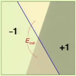
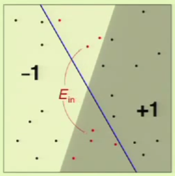
When the perceptron (the hypothesis) is changed, there is a huge amount of overlap:

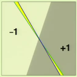
Only the area in yellow is what has changed between the two perceptrons; everything else overlaps.

Given this observation—that different hypotheses have significant amounts of overlapping with others—we would like to make the statement that one hypothesis exceeds epsilon often when another hypothesis exceeds epsilon.

Dichotomies

When counting the number of hypotheses, the entire input space is taken into consideration. In the case of a perceptron, each perceptron differs from another if they differ in at least one input point, and since the input is continuous, there are an infinite number of different perceptrons.

Instead of counting the number of hypotheses in the entire input space, we are going to restrict the count only to the sample: a finite set of input points. Then, simply count the number of the possible dichotomies. A dichotomy is like a mini-hypothesis, it’s a configuration of labels on the sample’s input points.

A hypothesis is a function that maps an input from the entire input space to a result:

The number of hypotheses $|\mathcal H|$ can be infinite.

A dichotomy is a hypothesis that maps from an input from the sample size to a result:

The number of dichotomies $|\mathcal H(\mathbf {x_1, x_2, \dots, x_N})|$ is at most $2^N$, where $N$ is the sample size. This makes it a candidate for replacing $M$.

Growth Function

The growth function counts the most dichotomies on any $N$ points.

This translates to choosing any $N$ points and laying them out in any fashion in the input space. Determining $m$ is equivalent to looking for such a layout of the $N$ points that yields the most dichotomies.

The growth function satisfies:

This can be applied to the perceptron. For example, when $N = 4$, we can lay out the points so that they are easily separated. However, given a layout, we must then consider all possible configurations of labels on the points, one of which is the following:

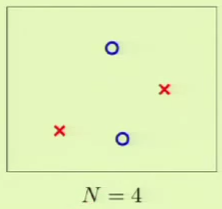
This is where the perceptron breaks down because it cannot separate that configuration, and so $\growthfunc(4) = 14$ because two configurations—this one and the one in which the left/right points are blue and top/bottom are red—cannot be represented.

For this reason, we have to expect that that for perceptrons, $m$ can’t be the maximum possible because it would imply that perceptrons are as strong as can possibly be.

We will try to come up with a hypothesis function that can easily determine the value of $m$.

Positive Rays

Positive rays are defined on $\mathbb R$ and define a point $a$ such that:

$\mathcal H$ is the set from the reals to a label $-1$ or $+1$, so $h\colon \mathbb R \to \{-1, +1\}$. Put more simply:

The dichotomy is determined by noticing between which two points in the input set $a$ falls into, these are the line segments between the input points on the line, of which there are $N + 1$, so:

Positive Intervals

Instead of a ray, we define an interval $[l, r]$ where any point that falls within it is defined as $+1$ and everything outside it is $-1$:

The way to vary the different dichotomies is by choosing two line segments—of which there are again $N + 1$—at which to place the interval ends. For this reason, the growth function is:

However, this doesn’t count the configuration in which the interval ends lie on the same line segment, making all points $-1$, so we add that:

Convex Sets

In this case, we take a plane and not a line so that $\mathcal H$ is the set of $h\colon \mathbb R^2 \to \{-1, +1\}$. In this model, if a point is found within a convex region then it results in $+1$, and $-1$ otherwise.

A convex region is a region where for any two points picked within a region, the entirety of the line segment connecting them lies within the region. For example, the left image is a convex region, but the one on the right isn’t because the line segment connecting the chosen two points doesn’t fall entirely within the region:

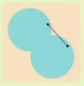
Convex regions can therefore be used to model dichotomies. The best layout for the points in the input set is to place them on the perimeter of a circle, in which case any configuration of the labels can be satisfied with a convex region as shown below:

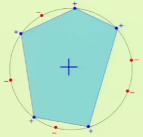
When a hypothesis set is able to reach every possible dichotomy, it is said that the hypothesis set shattered the points. This means that the hypothesis set is very good at fitting the data, but this is a trade off with generalization.

Break Point

What happens when $\growthfunc(N)$ replaces $M$? If the growth function is polynomial then everything will be fine. So we need to prove that $\growthfunc(N)$ is polynomial.

If no data set of size $k$ can be shattered by $\mathcal H$, then $k$ is a break point for $\mathcal H$. By extension, this means that a bigger data set cannot be shattered either. In other words, given a hypothesis set, a break point is the point at which we fail to achieve all possible dichotomies.

We already saw that for perceptrons, $k = 4$.

For positive rays where $\growthfunc(N) = N + 1$, the break point is $k = 2$ because $2 + 1 = 3$ and this is not the same as $2^2 = 4$. This is evidenced by the fact that the below configuration cannot be represented by a positive ray:

Similarly, for positive intervals where $\growthfunc(N) = \frac 1 2 N^2 + \frac 1 2 N + 1$, the break point is $k = 3$ because $\growthfunc(3) = 7 \not= 2^3 = 8$. The following configuration is an example configuration that cannot be represented by a positive interval:

Convex sets don’t have a break point, so $k = \infty$. Having no break point means that $\growthfunc(N) = 2^N$.

On the other hand, if there is a break point, then $\growthfunc(n)$ is guaranteed to be polynomial (growth) on $N$. This means that it is possible to learn with the given hypothesis set.

For example, consider a puzzle where there are three binary points $\mathbf x_1$, $\mathbf x_2$, and $\mathbf x_3$. The constraint is that the breaking point is $k = 2$, this effectively means that no combination of 2 points can be shattered, which in this context means that no two points can hold every possible combination: 00, 01, 10, and 11. A possible solution to the puzzle is:

$\mathbf x_1$	$\mathbf x_2$	$\mathbf x_3$
○	○	○
○	○	●
○	●	○
●	○	○

Theory of Generalization

We want to prove that $\growthfunc(N)$ is indeed polynomial, and also that it is therefore possible to use it to replace $M$.

First, to show that $\growthfunc(N)$ is polynomial, we will show that it is bound by a polynomial:

We will use the quantity $B(N, k)$ which is the maximum number of dichotomies on $N$ points with break point $k$. In other words, the maximum number of rows we can get on $N$ points such that no $k$ columns have all possible patterns

Conceptualization

To understand how $B(N, k)$ is defined, we should first determine each combination that is possible given a break point $k$ in a table with a column for every feature $\mathbf x_i$. We will then group these rows into two major groups.

$S_1$ is the group of $\alpha$ rows that are entirely unique on $\mathbf x_1$ to $\mathbf x_N$. If the last column $\mathbf x_N$ were removed, there would be no other row in the set with the same $\mathbf x_1$ to $\mathbf x_{N - 1}$.

Since there are $\alpha$ rows in $S_1$, we will say that $B(N, k)$ is defined in terms of it as:

$S_2$ is a group comprised of two subgroups: $S_2^+$ and $S_2^-$. The rows that belong here are those where, if the last row $\mathbf x_N$ were removed, there would be exactly one other row with the same $\mathbf x_1$ to $\mathbf x_{N - 1}$. If the last column is $-1$ then it goes into $S_2^-$ and vice versa. There are $\beta$ rows in $S_2^+$ and $\beta$ rows in $S_2^-$ for a total of $2\beta$ rows in $S_2$.

We can now add the extra term to $B(N, k)$:

Estimating $\alpha$ and $\beta$

We will now look at estimating $\alpha$ and $\beta$ by relating it to smaller numbers of $N$ and $k$ in order to achieve a recursive definition.

If we only focus on the columns $\mathbf x_1$ to $\mathbf x_{N - 1}$, then we can observe that the only unique rows are those in $S_1$ and those in one of the subgroups of $S_2$. This is relevant to $B(N, k)$ because it only concerns those rows that are different such that a condition occurs, the condition being:

We can make this relation because we are now considering $N - 1$ columns instead of all $N$, and we are still using a break point of $k$. We say “$\leq$” and not “$=$” as before because before, we made it equal by construction. However, we arrived at the mini-matrix of $\alpha + \beta$ rows in a manner where we can’t be positive that it maximizes the number of rows. However, we can be sure that it’s at most $B(N, k)$ because that is the maximum number that is possible.

Estimating $\beta$

We now want to estimate $\beta$ by itself. To do this, we’ll focus only on the $S_2$ group, comprised of $S_2^+ \cap S_2^-$ rows. Specifically, we’ll focus on a single mini-matrix of $\beta$ rows, such as $S_2^+$, without the last column $\mathbf x_n$. We will make the assertion that the break point for this mini-matrix is $k - 1$.

We can say this is true because, if it weren’t, then it would mean that it would indeed be possible to shatter $k - 1$ points within that mini-matrix. This would mean that we could attain $2^{k - 1}$ different rows within the mini-matrix; one for each different combination.

However, we must remember that we’re only focusing on one sub-matrix within the overall matrix. Further, we know that by definition there is another sub-matrix $S_2^-$ with the same amount of rows.

Therefore, if we then were to add back in the $\mathbf x_n$ column and also consider the rows from $S_2^-$, we would have $2^k$ rows with every possible combination (i.e. shattering $k$ points), which would contradict the fact that $k$ is the break point for the larger matrix. Therefore, we can be certain that the break point for the mini-matrix is at most $k - 1$. It could be lower, but since we are trying to achieve an upper bound, this is irrelevant.

With this in mind, we can define a relation for the maximum number of dichotomies within this mini-matrix which is composed of $N - 1$ points and for which we have proved that $k - 1$ is the break point:

Bound Relation

We want to arrive at an upper bound without having to know $\alpha$ or $\beta$.

If we combine the two derived relations into a system of inequalities:

Adding them together yields:

And since we know that:

We can say that:

Computing the Bound

To define this recursive bound, we will have to compute the values of the bound for smaller values of $N$ and $k$.

Numerical Derivation

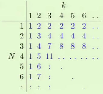
We can start doing this by filling out a table with the left hand side being $N$ and the top being $k$, where any element in the table specifies the maximum number of dichotomies for that combination $B(N, k)$. We begin doing this by filling out the bounds for when $k = 1$ and when $N = 1$.

When $k = 1$, we will only ever have one dichotomy because we’re using a binary function, since having more than one row would mean that one of the columns is fully exhausted.

When $N = 1$ and $k \geq 2$, given that we only have one point, the maximum number of dichotomies we can represent with a binary function is two.

With these bounds, we can then define every other point in the table:

Remembering that:

We can take an example such as $B(3, 3)$. To get this value, we add $B(N - 1, k - 1) = B(2, 2) = 3$, with $B(N - 1, k) = B(2, 3) = 4$, resulting in $B(3, 3) = 7$.

Analytical Derivation

A more analytic solution for computing the bound is given by the theorem:

We can easily verify that this is true for the boundary conditions that we derived in the table above.

For every other condition we must consider the induction step. Given the above theorem, it is implied that:

So it’s recursively implied that:

We can accomplish this by reducing the right hand side to resemble the left hand side:

We can reduce the final expression further by considering the example. You are in a room full of $N$ people, and want to determine how to choose $10$ people in the room: $\smash {N \choose 10}$. However, this can also be represented as the number of ways we can count $10$ people excluding you and including you; both cases are disjoint and together cover all combinations.

The number ways to choose $10$ people excluding you is $\smash {N - 1 \choose 10}$. It’s $N - 1$ because you are being excluded from the total number of people. The number of ways to choose $10$ people including you is $\smash {N - 1 \choose 9}$. It’s $9$ because you’re already being included, so you just need $9$ others. Adding these both together should therefore be the same as $\smash {N \choose 10}$.

So the above proves that the growth function $\growthfunc(N)$ is bounded by a polynomial $B(N, k)$. It’s polynomial because for a given $\mathcal H$, the break point $k$ is fixed.

To show that this holds, we can use it to determine the growth function $\growthfunc$ for:

• $\mathcal H$ is positive rays (break point $k = 2$):
  • $N + 1 \leq N + 1$
• $\mathcal H$ is positive intervals (break point $k = 3$):
  • $\frac 1 2 N^2 + \frac 1 2 N + 1 \leq \frac 1 2 N^2 + \frac 1 2 N + 1$
• $\mathcal H$ is 2D perceptrons (break point $k = 4$):
  • $\text {?} \leq \frac 1 6 N^3 + \frac 5 6 N + 1$

Vapnik-Chervonenkis Inequality

We would like to replace the $M$ factor in Hoeffding’s Inequality:

The following straightforward substitution would not work:

This is because we need to consider the following questions:

How does $\growthfunc(N)$ relate to overlaps? If we use the VC bound, it takes into consideration the various overlaps of the error.

What do we do about $\outsample$? The problem is that to determine the overlap we need to determine what a “bad point” is: a bad point is one that deviates from $\outsample$, so we need to know $\outsample$. Going back to the sheet with the holes analogy where we could only see the color of the points but not the separating line: to determine the error overlap between two separating lines, we would have to remove the covering sheet (the one with the holes).

We could alleviate this by getting rid of $\outsample$. To do this, we pick two samples instead of just one. We already know that $\outsample$ and $\insample$ track each other because $\insample$ is generated from the same distribution as $\outsample$. We give the two samples different names: $\insample$ and $\insample'$. Does $\insample$ track $\insample'$? It is obvious that each of them track $\outsample$, since they were generated from the same distribution, so consequently they do track each other, albeit perhaps more loosely.

The advantage of this fact is that, when considering multiple bins, the same situation applies. That is, with multiple bins, the tie between $\outsample$ and $\insample$ became looser and looser. Likewise, when considering two samples, they do track each other but it becomes looser and looser. The advantage of using two samples is that we are in the realm of dichotomies. We are in the realm of dichotomies because we now only care about what happens in the sample, not the input space, even though the sample is larger now at $2N$ not $N$.

With all of this in mind, the Vapnik-Chervonenkis Inequality is defined as:

The growth function is parameterized with $2N$ because we are now considering two samples. This inequality more or less says that we are making a statement that is probably (RHS), approximately (LHS epsilon), correct.

VC Dimension

The VC Dimension is a quantity defined for a hypothesis set $\mathcal H$ denoted by $\def \vc {d_{\text {VC}}} \vc(\mathcal H)$ and is defined as the most points that $\mathcal H$ can shatter; the largest value of $N$ for which $\growthfunc(N) = 2^N$.

Therefore, the growth function can be defined in terms of a break point $k$:

It can also be defined in terms of the VC dimension $\vc$:

With respect to learning, the effect of the VC dimension is that if the VC dimension is finite, then the hypothesis will generalize:

The key observation here is that this statement is independent of:

• the learning algorithm
• the input distribution
• the target function

The only things that factor into this are the training examples, the hypothesis set, and the final hypothesis.

VC Dimension of Perceptrons

We already know that $\vc = 3$ for $d = 2$ (2D). However, we would like to generalize this for any dimension. We will argue that $\vc = d + 1$. We prove this by showing that $\vc \leq d + 1$ and $\vc \geq d + 1$.

To do this we will first construct a set of $N = d + 1$ points in $\mathbb R^d$ in such a way that they can be shattered by the perceptron. We begin this by first setting the first element of every row vector to $1$ since it corresponds to $x_0$: the threshold weight which we have already established is always set to $1$. The rest of the rows are set so that they form an identity matrix which is easily invertible, which is a property that we will show to mean that every point can be shattered:

The key observation is that $\mathrm X$ is invertible.

The question is, can we find a vector $\mathbf w$ satisfying:

We can do this by changing the requirement to be:

This is valid because we’re using a binary function.

From here it’s a straightforward process to finding the vector $\mathbf w$ by isolating it, made possible by multiplying both sides by the inverse of the feature matrix $\mathrm X$, which we know is invertible because we specifically constructed it to be:

Since we were able to come up with $\mathbf w$, it means that we were able to shatter $d + 1$ points. More specifically, it means that we know for a fact that we can shatter at least $d + 1$ points, but it’s entirely possible that we can shatter more than that:

Therefore, to prove that $\vc = d + 1$, we must now show that $\vc \leq d + 1$, since the combination of both of these proofs would prove that $\vc = d + 1$. To prove that $\vc \leq d + 1$, we must show that we cannot shatter any set of $d + 2$ points.

For any $d + 2$ points $\mathbf {x}_1, \dots, \mathbf {x}_{d + 1}, \mathbf {x}_{d + 2}$, it is obvious that there are more points than dimensions. This is because each feature vector $\mathbf x_i$ is a $d + 1$ vector. Since there are more vectors than dimensions, we know that the vectors are linearly dependent; one of the vectors $\mathbf x_j$ can be represented in terms of the other $\mathbf x_i$ vectors:

It can be said that not all of the $a_i$ scalars are zeros, this follows from the fact that $x_0$ is always $1$.

Now consider the specific dichotomy where the vectors in $\mathbf x_i$ with a non-zero $a_i$ get the value $y_i = \text {sign}(a_i)$, the vectors with zero-valued $a_i$ get the value $\pm 1$, and the vector $\mathbf x_j$ gets the value $y_i = -1$:

We are going to argue that no perceptron can implement this dichotomy. Remember that $\mathbf x_j$ is the linear sum of the rest of the vectors $\mathbf x_i$, each scaled by a factor $a_i$. We now multiply them by a weight vector, in order to represent a perceptron:

An observation to make is that if by definition of the dichotomy, $\text {sign}(\mathbf w^{\mathrm T} \mathbf x_i) = \text {sign}(a_i)$, then it means that the signs of both are the same. By extension, this means that their product will always be greater than zero:

This by extension means that the sum of the $\mathbf x_i$’s will also greater than zero:

Therefore, since we defined $y_j = \text {sign}(\mathbf w^{\mathrm T} \mathbf x_j)$ in our dichotomy, the value of $y_j$ will always be:

However, in our dichotomy we defined $y_j$ as being equal to $-1$:

Therefore we cannot appropriately represent our dichotomy.

Now we have proved that $\vc \leq d + 1$ and $\vc \geq d + 1$. Therefore:

What is $d + 1$ in the perceptron? It is the number of parameters in the perceptron model: $w_0, w_1, \dots, w_d$. In essence, this means that when we have a higher number of parameters, we will have a higher $\vc$.

Interpretation of VC Dimension

The parameters in the weight vector correspond to degrees of freedom that allow us to create a specific hypothesis. The number of parameters correspond to analog degrees of freedom: varying any single parameter—which is itself continuous—yields an entirely new perceptron. The VC dimension translated these into binary degrees of freedom, since we’re only trying to get a different dichotomy.

This is important because it allows us to ascertain how expressive a model may be; how many different outputs we can actually get.

There is a distinction between parameters and degrees of freedom. This is because parameters may not contribute degrees of freedom.

For example, consider a 1D perceptron. This consists of a weight parameter and a threshold parameter, resulting in two degrees of freedom. This results in $\vc = d + 1 = 2$.

Now consider the situation where the output of this model is fed as input into another perceptron, which is fed to another perceptron and so on, for a total of four linked perceptrons. This corresponds to $8$ parameters since each perceptron contains $2$. However, there are still only $2$ degrees of freedom because every perceptron after the first simply returns the input; they are redundant.

For this reason, we can think of $\vc$ as measuring the effective number of parameters.

Minimum Sample Size

Knowing all this, we would like to find a way to determine the number of training points needed to achieve a certain level of performance. The first realization is that merely having a finite VC dimension means it’s even possible to learn. We should also remember that the VC inequality has two quantities that we would like to minimize: $\epsilon$ and $\delta$:

What we would like to do is say that we want a particular $\epsilon$ and $\delta$. For example, we would like to be at most 10% away from $\outsample$ ($\epsilon = 10\% = 0.1$) and we want that statement to be correct at least 95% of the time ($\delta = 5\% = 0.05$). How many examples do we need to satisfy these constraints?

The question is, how does $N$ depend on $\vc$? Consider a simplification of the RHS:

An observation made from plotting the above for increasing values of $d$ with $N$ vs the logarithm of the probability shows that $N$ is proportional to $\vc$. A practical observation made by machine learning academics and practitioners is that the actual quantity we are trying to bound follows the same monotonicity as the actual bound, e.g. a bigger VC dimension yields bigger quantities, if not close to proportional. The higher the VC dimension, the more examples that are required.

The rule of thumb is that for a large range of reasonable $\epsilon$ and $\delta$, and for a large range of practical applications, you need at least 10 times the VC dimension:

Generalization Bound

We will now simplify the VC inequality. We’ll begin by denoting the RHS as $\delta$:

We want to get $\epsilon$ in terms of $\delta$, to allow us to state the reliability $\delta$ of the statement we would like to achieve, and have the equation output the tolerance $\epsilon$ that the statement can guarantee with that reliability constraint.

This means that the probability that $\insample$ tracks $\outsample$ within $\Omega$ is at least $1 - \delta$:

The absolute value can be removed because $\insample$ is usually much smaller than $\outsample$, since $\insample$ is the value we minimize deliberately. The difference between $\outsample$ and $\insample$ is known as the generalization error:

This can then be rearranged and simplified further into the generalization bound:

The effect of the generalization bound is that it bounds the unknown value $\outsample$ by values we do know, namely $\insample$ and $\Omega$.

Bias-Variance Tradeoff

We have noticed that there is a trade off between approximation and generalization. In other words, we want to minimize $\outsample$, such that we attain a good approximation of $f$ out of sample. The more complex the hypothesis set $\mathcal H$, the better chance we have of approximating $f$. However, the less complex of a hypothesis set $\mathcal H$, the better the chance of generalizing out of sample.

We have already learned that VC analysis is one approach of decomposing $\outsample$:

Bias-Variance analysis is another approach to decomposing $\outsample$, which does so into two components:

• how well $\mathcal H$ can approximate $f$
• how well we can zoom in on a good $h \in \mathcal H$

Bias-Variance applies to real-valued targets and uses squared error.

$g^{(\mathcal D)}$ refers to the fact that the hypothesis comes from the dataset $\mathcal D$.

Given a budget of $N$ training examples, we want to generalize the above for any data set of size $N$:

We’re only going to focus on the inner component of the RHS. We’re going to consider the concept of an average hypothesis $\def \avghypo {\bar g} \avghypo$ so that:

The average hypothesis for a particular point $\mathbf x$, $\avghypo(\mathbf x)$, is equivalent to finding the hypothesis found from many different data sets, then averaging the result of each of those hypothesis on the point $\mathbf x$:

Bias-Variance Representation

We will now decompose the expected error into two components, bias and variance:

The result is an equation that says that the expected error $\mathbb E_{\mathcal D}$ for a particular data set $\mathcal D$ given the hypothesis $g^{(\mathcal D)}(\mathbf x)$ resulting from that given data set is measured against the actual target function $f(\mathbf x)$, and that error measure is equivalent to the variance—the expected error of the hypothesis $g^{(\mathcal D)}(\mathbf x)$ measured against the average hypothesis $\bar g(\mathbf x)$, plus the bias—the error measure of the average hypothesis $\bar g(\mathbf x)$ against the target function $f(\mathbf x)$:

Both the bias and the variance in the above equation are as measured from a particular point $\mathbf x$. The bias essentially represents the bias of the hypothesis set $\mathcal H$ away from the target function. The variance is essentially measuring the effect of the finite data set, where each finite data set will vary in its result. Therefore:

Tradeoff

There is a trade off between the bias and the variance:

If we go from a small hypothesis to a bigger one, the bias goes down but the variance goes up:

We can now formulate the relations between the hypothesis for a given dataset $\mathcal D$ known as $g^{(\mathcal D)}(\mathbf x)$, the average hypothesis $\bar g(\mathbf x)$, and the target function $f(\mathbf x)$:

We will now use an example to prove that this is true. Given a target function that is a sinusoid:

We are only given two examples $N = 2$. There are two hypothesis sets, one is a constant model and the other one is linear, and we would like to see which one is better:

We will now see which one fares better by approximating what we think would be the best hypothesis from each set. In the case of the constant model, we would choose the line at $y = 0$ to minimize the MSE. The linear model would use a line that also tries to minimize the MSE. The following is the $\outsample$ for both:

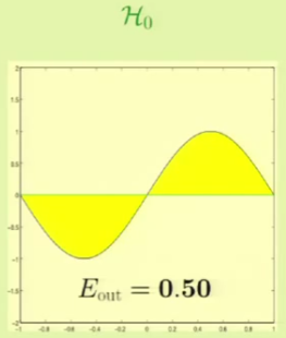
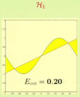
It’s clear that from approximation, $\mathcal H_1$ seems to be better. We will now see which one fares better through machine learning. For example, for these particular two points we get the following result:

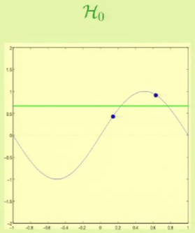
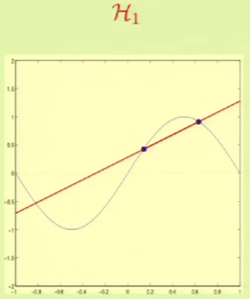
The problem is that these results depend on the two points that we were given, so it complicates the task of comparing the two hypothesis sets. This is why we need bias-variance analysis, it gives us the expected error with respect to the choice of the data set.

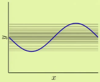
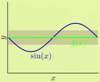
If we were derive a hypothesis from any two points, for a large number of different two points, we would come up with something like the left image, where every line represents a derived hypothesis. It therefore stands to reason that the average hypothesis would fall somewhere near $y = 0$—the midpoint of the range of possible hypotheses. The error measure of the average hypothesis against the target function is the bias, and the variance is represented by the gray region which corresponds to the standard deviation of the possible hypotheses. It’s apparent that this model has a high bias ($0.5$) and a low variance ($0.25$):

The same is slightly more complicated with the second hypothesis $\mathcal H_1$ because of its linear model, which yields very different hypotheses, that is, high variance ($1.69$). There is low bias ($0.21$) however, because it has many different hypotheses to average from:

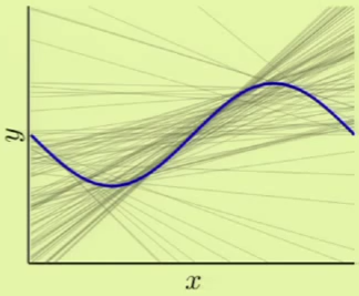
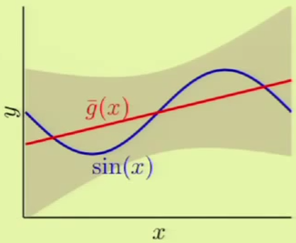
It’s clear that when the two components are summed for both models, the expected error of the first hypothesis set $\mathcal H_0$ is much lower than $\mathcal H_1$’s.

The conclusion from this example is that we are matching the model complexity to the data resources, not to the target complexity.

Learning Curves

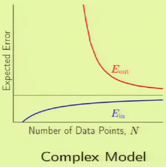
A learning curve plots the expected value of $\outsample$ and $\insample$ as a function of $N$. For a data set of size $N$, how does the expected $\outsample$ and expected $\insample$ vary with $N$?

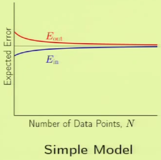
The following images are learning curves for a simple and complex model. The simple model shows that $\outsample$ decreases with the $N$, but so does $\insample$, which can be attributed to exceeding the degrees of freedom available in the hypothesis set. The second model has so many degrees of freedom that it can fit the training set perfectly until the part where the blue curve appears on the left side, however, $\outsample$ is very high before that point, which corresponds to not learning anything; just memorizing the examples. Therefore if there are very few examples, then it’s clear that the simple model would fare better. This is why we want to match the model’s complexity to the data resources that we have.

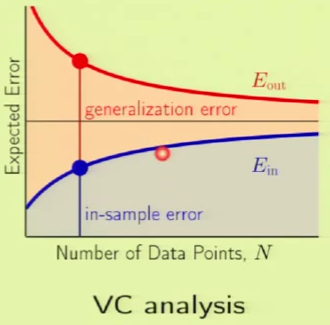
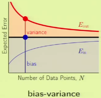
The following is a comparison of the learning curves for a given model using VC analysis and bias-variance analysis. In the VC analysis curve on the left, the blue region is $\insample$ and the red region is $\Omega$—what happens within the generalization bound. In the Bias-Variance curve, the black bar is the approximation. Everything below the approximation is the bias, so everything else under the $\outsample$ curve must be the variance. Both curves are talking about approximations. The Bias-Variance curve is concerning over-all approximation, whereas the VC analysis curve is concerning in-sample approximation.

Analysis of Linear Regression

Given a data set $\mathcal D = \{ (\mathbf x_1, y_1), \dots, (\mathbf x_n, y_n)\}$ and a noisy target function:

The linear regression solution is:

The in-sample error vector would be:

The ‘out-of-sample’ error vector would be calculated by generating a new set of points from the same inputs but with different noise and would therefore be:

This yields the following analysis learning curve. Up until $d + 1$ data points, the data was being fit perfectly. The best approximation error, the variance of the noise, is denoted by $\sigma^2$.

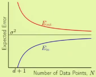
We can observe the following characteristics:

Linear Model II

Non-Linear Transformations II

To recap, a transformation $\Phi$ transforms the input vector $\mathbf x$ to the feature space, resulting in a feature vector $\mathbf z$, where every element $z_i$ is the result of performing a non-linear transformation $\phi_i$ on the entire input vector. Therefore, $\mathbf z$ can be of different size, often longer, than the input vector $\mathbf x$:

It’s important to remember that the final hypothesis $g(\mathbf x)$ will always be in the $\mathcal X$-space; the $\mathcal Z$-space is transparent to the user.

What is the price paid in using a non-linear transformation? Well it has been established that the VC dimension of a $d + 1$ sized input vector is $d + 1$, therefore the feature vector $\mathbf z$, whose size is $\tilde d + 1$, will have a VC dimension of at most $\tilde d + 1$, where $\tilde d$ is generally larger than $d$. It’s “at most” because the VC dimension is always measured in the $\mathcal X$-space, and this is the $\mathcal Z$-space. While this means that we will be able to better fit the data, we won’t have much of a chance of generalization.

For example considering the following case 1 where there are two outliers in the data set. If we want to really fit the data, we could use a 4th-order surface in order to completely classify the data in the set. However, this increase in complexity would mean that it’d be very difficult to generalize. Sometimes it’s best to accept that there will be an $\insample > 0$.

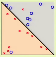
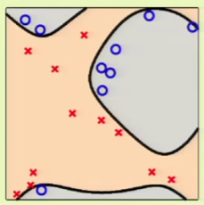
Now consider case 2, where we don’t stand a chance using a linear model to fit the data, which clearly falls inside a circular region:

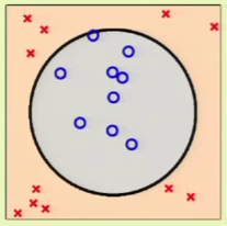
In this case, we can use a non-linear transformation to map the data to a general 2nd-order surface as follows:

Note that with $\mathbf x$ we were only using three weights, however in $\mathbf z$ we are using six weights. This effectively translates to now requiring twice as many examples to achieve the same level of performance. So a natural conclusion is to try to find a way to avoid paying this increase in cost.

First let’s consider the following alternative model, since it seems we only need $x_1^2$ and $x_2^2$ to represent the circle. Now we only have three weights again, the same as with the linear model represented by $\mathbf x$:

We reduce the cost further by adopting the following model, which does away with representing the independence of $x_1^2$ and $x_2^2$, as they simply represent the radius:

Now consider the extreme case, where we completely reduce to a single parameter, completely doing away with the threshold weight:

The problem with these reductions is that the guarantee of the VC inequality is forfeited if we look at the data. We can consider the concept of us simplifying the model for the machine as performing a hierarchical learning process, where we the human do some learning, and then pass the result for the machine to finish the learning process. From this perspective, it’s apparent that the VC dimension resulting from this process is that of the entire hypothesis space that we as the human considered during the simplification process.

The bottom line is that looking at the data before choosing the model can be hazardous to your $\outsample$. The act of looking at the data before choosing the model is one of the many mistakes that fall under data snooping.

Logistic Regression

We’re already familiar with two linear models. The first is linear classification which classifies data points based on what side of a hyperplane they’re on. The second is linear regression, which makes it straightforward to predict a regression, and is computed by skipping the last step of linear classification, the part where it determines the sign of the result.

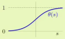
A third model called logistic regression can predict the probability of an event occurring, and is defined as:

Where $s$ is simply the dot product of the weight and feature vectors as is done in the other two linear models, and $\theta$ is a non-linear function that is often called a sigmoid, and looks something like this:

In our particular case, the formula we’re going to use is:

This kind of function is also called a “soft threshold,” since it’s a gradual increase rather than a hard increase as in linear classification. It is in this way that this kind of function expresses uncertainty.

Given this functions’ bounds $(0, 1)$ and the fact that it’s a “soft threshold,” it’s clear that it can be interpreted as a probability. For example, when predicting heart attacks, we want to predict whether there’s a small or big risk in having a heart attack anytime soon. If we used a binary function as in linear classification, it would be too hard of a threshold and thus wouldn’t really convey as much meaningful information, since it isn’t clear exactly which things definitely cause heart attacks.

On the other hand, with a logistic regression model, we could predict the probability of having a heart attack in the next 12 months. In this context, the dot product between the weight and feature vector can be considered a “risk score,” which can give one a general idea of the result but which must still be passed through the logistic function in order to determine the probability.

A key point is that this probability is considered as a genuine probability. That is, not only does the logistic function have bounds of $(0, 1)$, but that the examples also have a probabilistic interpretation. For example, the input data consists of feature vectors and binary results. It’s clear that there is some sort of probability embedded in yielding the binary results, but it is unknown to us. Therefore it can be said that the binary result is generated by a noisy target:

So the target $f$ is:

And we want to learn $g$:

Logistic Regression Error Measure

We have established that for each data point $(\mathbf x, y)$, $y$ is generated by the probability $f(\mathbf x)$. The plausible error measure is based on likelihood, that is, we are going to grade different hypotheses according to the likelihood that they are actually the target that generated the data. In other words, we are going to assume that a given hypothesis is indeed the target function, and then we will determine how likely it is to get a given result from its corresponding feature vector. Expressed mathematically:

Now substitute $h(\mathbf x)$ with $\theta(\weightT \feature)$, while noting that $\theta(-s) = 1 - \theta(s)$, since:

So now we can simplify the probability to:

Now we can determine the likelihood of the entire data set $\mathcal D = (\feature_1, y_1), \dots, (\feature_N, y_N)$ is:

It’s noteworthy to observe that the same weight vector is being used for each of those products, so that if it’s varied to better fit one particular data point, it might no longer fit another. Therefore, whatever maximizes this product would represent the likelihood that the weight vector is representing the underlying probability distribution.

So now we want to see how to maximize the likelihood with respect to $\weight$. This corresponds to minimizing the error:

Logistic Regression Learning Algorithm

Now that we have the learning model and error measure we can define the learning algorithm. Compared to the closed-form solution from the other two models, we will have to use an iterative solution called gradient descent, which is a general method for non-linear optimization.

Gradient descent starts at a point on the error function and iteratively takes steps along the steepest slope towards the minimum. So we’ll have a direction unit vector $\hat v$ pointed in the direction of the steepest slope and a fixed step size $\eta$ which we will define as being small since we want to approximate the surface using the first order expansion of the Taylor series—the linear approximation—which works best when the distance between the two points is small. With this in mind, the new position after a step can be expressed as:

To derive the direction unit vector $\hat v$, we first observe that the change in the value of the error is simply the difference between the error at the new point and the error at the original point:

Remembering that the Taylor series is defined as:

Then the first-order approximation is defined as $n = 1$ so that the series is:

If we drop the remainder term $R_2$, then we are left with the linear approximation:

Therefore, for $f(x + a)$ it is defined as:

This representation of the linear approximation is similar to our definition of the change in the value of the error between the two positions:

However, we don’t want to use the linear approximation just yet. There’s another concept known as the gradient which basically defines a vector field so that at any given point in the space, a vector is available at that point which points in the direction of the “steepest ascent.” The gradient is simply defined as the vector of all of the possible partial derivatives. For example, given a function:

The gradient is denoted by the $\nabla$ symbol and is defined as:

It’s obvious how the gradient can be useful here. It provides us with a way to determine—at any point on the surface—in what direction to move to go deeper towards the minimum. This is possible by finding the gradient vector—which points in the direction of the “steepest ascent”—and negate it so that it then points in the direction of the “steepest descent”. This is clearly useful, and fortunately there is a similar linear approximation to a vector-taking function for a gradient:

This means that for $f(\mathbf x + \mathbf x_0)$:

So we can replace the RHS with the dot product of the gradient and the unit vector $\hat v$ ¹:

Since we know that $\hat v$ is a unit vector, we know that regardless of the value of $\hat v$, the inner product between $\nabla \insample(\mathbf w(0))$ and $\hat v$ cannot exceed the norm $\lVert \nabla \insample(\mathbf w(0)) \rVert$, be it in the positive or negative direction. Therefore we can guarantee that $\Delta \insample$ must be greater than or equal to the negative norm:

We would therefore like to choose $\hat v$ that is closest to this lower bound, since we want to minimize the error, and a negative change in error corresponds to a big decrease in error, and therefore descending rapidly. Since $\hat v$ is by definition a unit vector, we can simply take the gradient itself and divide it by its norm to normalize it, then negate it to flip from ascent to descent.

The above implies a fixed step. We could instead adopt a step distance based on the slope of the current position, easily accomplished by scaling the direction vector $\hat v$ by the norm of the gradient at the current position. This allows the algorithm to take bigger steps in steeper locations, and take smaller steps once it begins to near the minimum. In this case, $\eta$ now refers to the “learning rate”:

Now that we have all of the pieces we can construct the learning algorithm:

1. initialize the weights at $t = 0$ to $\weight(0)$
2. for $t = 0, 1, 2, \dots$ do

   1. compute the gradient

      $$ \nabla \insample = - \frac 1 N \sum_{n = 1}^N \frac {y_n \feature_n} {1 + e^{y_n \weightT(t) \feature_n}} $$

   2. update the weights: $\weight(t + 1) = \weight(t) - \eta \nabla \insample$

   3. repeat until it is time to stop

3. return the final weights $\weight$

To recap the three linear models we’ve learned so far, here is a table for their possible uses within the context of credit analysis:

task	model	error measure	algorithm
approve or deny	perceptron	classification error	PLA, Pocket, …
amount of credit	linear regression	squared error	pseudo-inverse
probability of default	logistic regression	cross-entropy error	gradient descent

Neural Networks

Stochastic Gradient Descent

Gradient descent minimizes $\insample$ by iterative steps $\Delta \weight$ along $- \nabla \insample$, and each one of those steps occurs only after a full epoch, where an epoch marks the event of having examined all of the examples. Instead of being restricted to taking steps only after having examined all of the examples, we would like to try to adapt it so that it can perform a step after having considered a single random example. This modified gradient descent is known as stochastic gradient descent, whereas comparatively the “original” gradient descent will be referred to henceforth as batch gradient descent because it performed a step $\Delta \weight$ only after having examined all of the examples.

This is accomplished by performing epochs until a tolerance is met, where each epoch consists of examining every single example in a random order, and for every example considered, recomputing the gradient based on that example alone and descending along its negative direction. Compare this to batch gradient descent, which had to compute the gradient based on all of the points and summing up the result.

1. until desired tolerance is met
   1. (epoch) for every example considered in a random order
      1. perform a descent along the negative of the gradient which was computed for that example

Stochastic gradient descent is a randomized version of gradient descent, where we pick one example $(\feature_n, y_n)$ at a time and apply gradient descent based on $\crossentropy(h(\feature_n), y_n)$, similar to PLA. It’s expected that this is similar to performing the descent by considering every single point:

There are a variety of benefits of SGD. One is that it is a cheaper computation, because we can make a move, or descent, after having considered one point instead of every single point. Another advantage is randomization which can help in escaping very shallow local minima or certain flat regions that precede the actual minimum. Finally, SGD is a very simple optimization, so it is widely used and a variety of “rules of thumb” have been formulated. For example, one rule of thumb is to start with a learning rate of $\eta = 0.1$ and scale it from there.

For example, think back to the movie ratings model which can learn to suggest movies to users based on their tastes. The user $i$’s vector $\mathbf u$ consists of tastes $u_1, u_2, \dots, u_k$ in different movie qualities, the movie $j$’s vector $\mathbf v$ corresponds to how well a movie represents each of those qualities $v_1, v_2, \dots, v_k$ in the feature vector, and the result $r_{ij}$ is the movie rating.

We can take the dot product between the user and movie vector as a measure of how well both agree with each other, in fact, this will correspond to the rating. Therefore, the error measure can be represented as the difference between the actual rating and the computed rating:

Neural Network Model

The perceptron model has a break point of 4 because it couldn’t properly model situations such as the following:

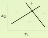
Although the above can’t be modeled with one perceptron, perhaps the combination of more than one perceptron can. For example, we could divide the space twice, independently, with two different perceptrons and then somehow combine their results to effectively model the above scenario:

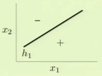
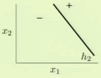
The results of these two independent perceptrons can be combined to model the impossible scenario. Specifically, one way this can be accomplished is by modeling logical AND and OR operations to combine results of separate perceptrons.

Logical OR can be modeled as a perceptron where the threshold weight $x_0$ is set to $1.5$. This way it’ll only return $-1$ if both of the other features are $-1$, as is expected of logical OR:

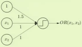
Logical AND can be modeled as a perceptron where the threshold weight $x_0$ is set to $-1.5$. This way, both of the other features have to be $+1$ in order to overcome the threshold weight and thus return $+1$, just as with logical AND:

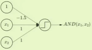
With these models, we can model the original complicated scenario. We can take the AND result of one of the perceptrons such as $h_1$ and the negation of the other perceptron, $h_2$. This essentially means that the bottom quadrant in the target model would be $h_1$’s + AND the negation of $h_2$’s - which results in + as in the target model. The left quadrant can similarly be modeled by taking $h_1$’s - AND the negation of $h_2$’s - which results in - as in the target model. We take this and OR it with the alternate scenario, where $h_1$’s values are negated, to fully complete the model.

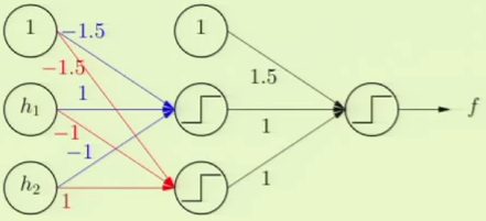
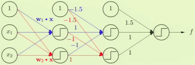
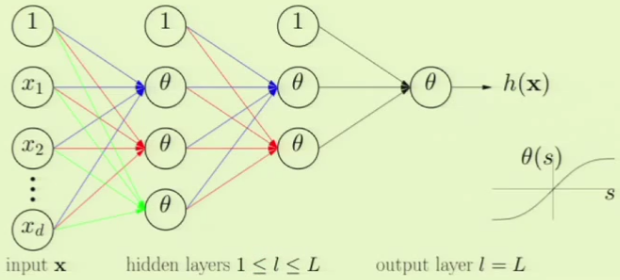
The full, multi-layer perceptron can now be constructed, with the additional layer at the beginning which yields the separate, independent perceptrons $h_1$ and $h_2$. Note that there are three layers, and it is strictly “feedforward,” that is, we don’t feed outputs to previous layers nor do we skip layers:

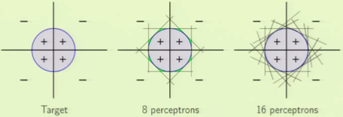
This new model seems very powerful, with a seemingly infinite degree of freedom able to model a variety of situations. For example, we can model a circle only using perceptrons instead of using a non-linear transformation as we did before. The more perceptrons we use, the better the approximation:

There are two costs that this seemingly powerful model can incur. The first is generalization because we have so many perceptrons, yielding a higher VC dimension and with it higher degrees of freedom. This is a problem, but at least being aware of it means that we can overcome it by simply using an adequate number of examples. The other, perhaps more important cost, is that of optimization. When the data is not separable, it becomes a combinatorial optimization problem that is very difficult to solve.

The problem of optimization can be solved by using soft thresholds instead of the hard thresholds found in perceptrons. This can be facilitated with gradient descent, which features soft thresholds. Once the solution is found with soft thresholds and as a result so are the weights, we can switch to hard thresholds to perform classifications.

A neural network has various inputs and layers. Each layer has a non-linearity $\theta$, which is a generic non-linearity—not specifically the logistic function in logistic regression. To be precise, the non-linearity $\theta$ is similar to the logistic function except that it ranges from $-1$ to $+1$, to better approximate the hard threshold that goes from $-1$ to $+1$. Each of the non-linearities $\theta$ can be different. A famous approach to take is to make all of the $\theta$’s be non-linear and then make the final $\theta$ actually be linear. The intermediate layers are referred to as hidden layers. The final layer is referred to as the output layer:

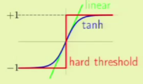
The non-linearity $\theta$ in the neural network is the hyperbolic $\tan$, the $\tanh$ function which takes on values ranging from $(-1, +1)$. If the signal (sum of the weights) is small then the $\tanh$ function acts linear, and otherwise if it is very large then it asks as a hard threshold:

The parameters of the neural network are weights $w$ indexed by three indices consisting of the layers, inputs, and outputs, and each of these indices take on the following ranges:

The neural network can therefore be represented by a recursive definition:

The neural network is then constructed by applying the feature vector $\feature$ to the first layer in the neural network $x^{(0)}_1, \dots, x^{(0)}_{d^{(0)}}$ such that it eventually ends up in one scalar valued output from the last layer $\smash {x^{(L)}_1}$, which is the value that we will say that $h(\feature)$ produces.

Neural Network Backpropagation

We will now apply stochastic gradient descent to our neural network. With SGD, whenever an example passes through the neural network, we will adjust all of the weights in the network in the direction of the negative of the gradient of that single example.

Therefore it can be said that all of the weights $\weight = \{ w^{(l)}_{ij} \}$ determine $h(\feature)$. We then get the error on the example $(\feature_n, y_n)$ which is defined as $\crossentropy(h(\feature_n), y_n) = \crossentropy(\weight)$. Therefore, to implement SGD we need to obtain the gradient $\nabla \crossentropy(\weight)$:

There is a trick for efficient computation of the gradient by using the chain rule to separate the partial derivative into two separate partial derivatives:

This is easily observable when we look at a diagram of a neural network layer:

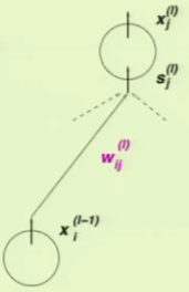
We already know the second component’s result:

Now we only need to determine the value of the first component, which we will refer to as $\smash {\delta^{(l)}_j}$. This component would be easiest to compute if we knew the error output itself, for this reason, we will first compute it at the last layer and then propagate it backwards throughout the rest of the neural network. So what we want is $\smash {\delta^{(L)}_1}$, but first we’ll have to define $\crossentropy(\weight)$ for the final layer:

The output of the neural network is simply the signal of the final layer passed to that layer’s non-linear function $\theta$:

Due to the chain rule, we have to know the derivative of $\theta$ in order to compute the partial partial derivative $\delta$:

Now all that we have to do is back-propagate the final layer’s $\delta$ to the previous layers. This is again facilitated by using the chain rule to break the partial derivative up into multiple components:

This decomposition into three components is again observable from a diagram of a neural network layer:

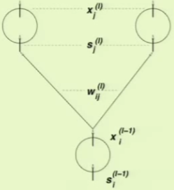
When the backpropagation is complete, there will be $\delta$ values available at every position in the network where there is an $s$ value. The algorithm can now be formulated:

1. initialize all weights $w^{(l)}_{ij}$ at random
2. for $t = 0, 1, 2, \dots$ do
   1. pick $n \in \{ 1, 2, \dots, N\}$
   2. forward: compute all $x^{(l)}_j$
   3. backward: compute all $\delta^{(l)}_j$
   4. update the weights: $w^{(l)}_{ij} \gets w^{(l)}_{ij} - \eta x^{(l - 1)}_i \delta^{(l)}_j$
   5. repeat until it is time to stop
3. return the final weights $w^{(l)}_{ij}$

One final intuition is that the hidden layers are performing non-linear transformations which produce higher order features. However, these are features learned by the learning algorithm, with the VC dimension already taken into account. This allows us to avoid looking at the data to determine a proper non-linear transformation to perform explicitly and manually.

Overfitting

Imagine that we are given five points along with the target function in blue. We can see that the target function doesn’t exactly fit some of the points, which means that there is some noise involved. If we were then to use a 4th-order polynomial, such as the one in red, to fit the points perfectly, we would get a very large $\outsample$ despite $\insample = 0$.

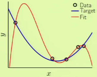
Overfitting is the act of fitting the data more than is warranted. It is a comparative term used to express that a solution went past a desirable point in terms of fitting, more so than another solution, where the different solutions can be different instances within the same model or different models entirely. For example, if we had used a 3rd-order polynomial instead, we would not have achieved $\insample = 0$ but $\outsample$ would have been considerably less. In that case, the 4th-order solution could have been considered overfitting compared to the 3rd-order solution. In other words, there is a distinction between overfitting and just plain bad generalization.

Overfitting within the same model occurs when $\insample$ is decreasing but $\outsample$ is beginning to increase, that is, when both error measures begin to diverge:

If we stop right before this occurs, we call it early stopping:

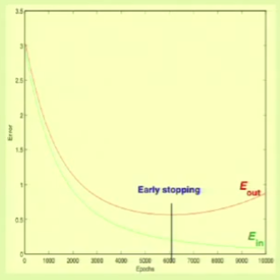
The main culprit cause for overfitting is fitting the noise, which is a natural side-effect of fitting the data. Fitting the noise is harmful because the learning algorithm is forming its solution from it, trying to detect a pattern, and therefore “hallucinating” an out-of-sample solution extrapolated from the in-sample noise.

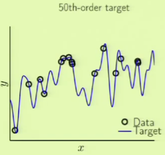
Consider two different target functions with accompanying data points. The first target on the left is a simpler 10th-order polynomial but has noise involved (noisy low-order target), whereas the one on the right is a more complicated 50th-order polynomial but is noiseless (noiseless high-order target):

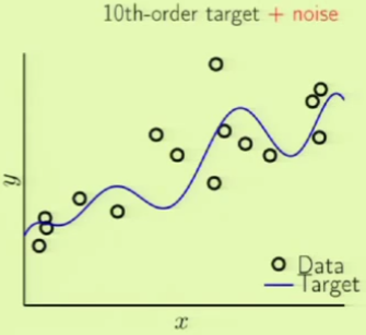
If we try to model the first target function using two models, a 2nd and 10th-order polynomial, we get this result:

The error measures clearly show that the 10th-order fit is a case of overfitting, showing the effects of how the 10th-order fit bends itself just to fit noise:

error	2nd-order	10th-order
$\insample$	$0.050$	$0.034$
$\outsample$	$0.127$	$9.00$

Now we can try using the same order fits to model the second target function. Remember that the target is a 50th-order polynomial:

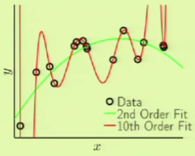
In this case, the 10th-order polynomial can fit the sample data very well, but the out of sample error is even worse. This is clearly another case of overfitting, because this target function actually does have noise, but it isn’t the usual kind of noise:

error	2nd-order	10th-order
$\insample$	$0.029$	$10^{-5}$
$\outsample$	$0.120$	$7680$

In the case of the 10th-order target, we can think of the 2nd-order fit as learner $R$ (for restricted) and the 10th-order fit as learner $O$ (for overfit). It can be said that $O$ chose $\mathcal H_{10}$ because it knew that the target is a 10th-order polynomial. On the other hand, $R$ chose $\mathcal H_2$ because it considered the number of points available in the training set, $15$. Choosing a 2nd-order polynomial provides three parameters, such that the ratio of points to degrees of freedom is 5:1, so we’re pushing our luck since we know the rule of thumb is for it to be 10:1, but we do so because we figure we can’t use a simple line when we know that the target is a 10th-order polynomial.

This reinforces the guideline that we are trying to match the data resources rather than the target complexity.

In the case of the 50th-order polynomial, $O$ chooses $\mathcal H_{10}$ and $R$ chooses $\mathcal H_2$. We still got bad performance out of sample with $O$, so is there really no noise?

Role of Noise

We will conduct an experiment to observe the effects of overfitting, specifically to observe the impact of noise level and target complexity. Consider the general target function with added noise:

The level (energy) of noise is denoted by $\sigma^2$. This is a higher order $Q_f$ (target complexity) polynomial. We normalize the polynomial quantity such that the energy is always $1$, since we want to observe the signal-to-noise ratio (SNR), so that we can definitively say that $\sigma^2$ is really the amount of noise.

This function doesn’t generate very interesting polynomials, so we will instead use the coefficients of Legendre polynomials, which are simply polynomials with specific coefficients such that from one order to the next they are orthogonal to each other, similar to harmonics in a sinusoidal expansion. Once the noise is added, the polynomial formed will be more interesting.

Those factors that seem to affect overfitting are the noise level $\sigma^2$, the target complexity $Q_f$, and the data set size $N$.

We fit the data set $(x_1, y_n), \dots, (x_N, y_N)$ using our two models $\mathcal H_2$ and $\mathcal H_{10}$, 2nd-order and 10th-order polynomials respectively. Each model yields a hypothesis function $g_2 \in \mathcal H_2$ and $g_{10} \in \mathcal H_{10}$. The overfit measure is then defined as the difference between $\outsample$ for the more complex model’s hypothesis $g_{10}$ and $\outsample$ for the simpler model’s hypothesis $g_2$. This works because if the more complex model is overfitting, its out of sample error will be bigger, yielding a larger positive number. If instead the measure yields a negative number, then it shows that the complex model is not overfitting because it’s performing better than the simpler model:

If we run an experiment for tens of millions of iterations (complete runs). The following plots show the impact of the noise $\sigma^2$ and the complexity $Q_f$ on the overfit measure based on the data set size $N$:

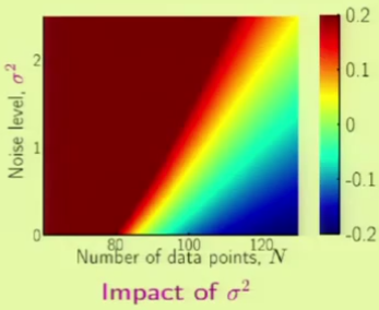
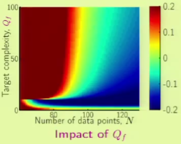
The main takeaway from these results is that there seems to be another factor aside from “conventional noise” that affects overfitting. The truth is that the noise $\sigma^2$ measured in the left image is called stochastic noise (the more conventional noise). Meanwhile, the effect observed in the right image which seems to be related to an increase in complexity that brings about a higher overfit measure is caused by deterministic noise.

Deterministic Noise

Deterministic noise is the part of $f$ that the best hypothesis function $h^*$ from $\mathcal H$ cannot capture:

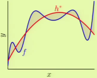
An example of why we call this noise is the following. Imagine a younger sibling that has just learned fractions in school and comes to you to ask you to tell them more about numbers. You begin to teach them about negative numbers and real numbers, in a basic sense, but you probably would be better off not telling them about complex numbers. The reason is that this would be considered completely noise from their perspective, their “hypothesis set” would be so small that if you told them about complex numbers, they would create a pattern that doesn’t actually exist (fitting the noise). You’d be better off not telling them about complex numbers in order to avoid misleading them (just as noise would in learning).

This is why if we have a hypothesis set and part of the target function that we can’t capture, there’s no point in trying to capture it, because then we would be detecting a false pattern which we cannot extrapolate given the limitations of the hypothesis set.

Deterministic noise differs from stochastic noise in that:

1. it depends on hypothesis set $\mathcal H$; for the same target function, using a more sophisticated hypothesis set will decrease the deterministic noise
2. it’s fixed for a given $\feature$

When we have a finite $N$ set, we gain the unfortunate ability to fit the noise, be it stochastic or deterministic, which wouldn’t be possible if we had an infinite sized set.

Noise and Bias-Variance

Remember that the bias-variance decomposition concerned a noiseless target $f$. So how would the decomposition work if $f$ were a noisy target?

We can decompose it into bias-variance by adding a noise term:

Form this, we can derive the two noise terms. These can be described as moving from your hypothesis to the best possible hypothesis (variance), from the best possible hypothesis to the actual target (bias), and finally from the target to the actual output (with noise added):

Notice that the bias consists of the deterministic noise. This is because the average hypothesis $\bar g(\feature)$ is supposed to be about the same as the best hypothesis, so the bias is a measure of how well the best hypothesis can approximate $f$, which is effectively a measure of the energy of deterministic noise.

Dealing with Overfitting

There are two cures for overfitting. Regularization can be described as hitting the breaks to avoid going into the point of overfitting. Validation on the other hand involves checking the bottom line and making sure it doesn’t overfit.

Regularization

Regularization tends to reduce the bias at the expense of slightly increasing the variance. Regularization can be thought of as providing intermediate levels between the different fits such as constant, linear, quadratic.

Polynomial Model

The model $\mathcal H_Q$ consists of the polynomials of order $Q$. A non-linear transformation produces $\mathbf z$ by taking a scalar $x$. In effect, the elements in $\mathbf z$ correspond to the coefficients of the Legendre polynomials. The parameterization of the hypothesis set is therefore represented as the linear combination of the weights and the Legendre polynomial coefficients:

The Legendre polynomials denoted by $L_q$ look like this:

Because of the summation, we’re going to apply linear regression in the $\mathcal Z$-space.

We’ve already placed a hard constraint on the weights in the previous section, in which case $\mathcal H_2$ was the constrained version of $\mathcal H_{10}$. This is represented in the polynomial model by having set $w_q = 0$ for $q > 2$.

However, we’d like more of a softer constraint. Given a budget $C$ for the total magnitude squared of the weights, $w_q^2$. Instead of the harder constraint above where we outright set some of the weights to $0$, we just want them to be generally small. This can be thought of as a soft-order constraint:

Given this model, we now want to minimize $\insample$ while being subject to the constraint (shown in vector form):

The solution will be called $\def \weightreg {\weight_{\text {reg}}} \weightreg$, which signifies regularization, as opposed to $\def \weightlin {\weight_{\text {lin}}} \weightlin$ which signifies linear regression.

The solution can be visualized by an ellipsoid. The in-sample error $\insample$ is represented by the blue ellipsoid. The boundary of the ellipsoid consists of the same value for $\insample$. Anything inside the boundary is a smaller value and outside is larger. The value of $\weightT \weight$ is represented by the red ellipsoid, so the constraint means that we have to be inside the red ellipsoid. The solution given by linear regression $\weightlin$ is at the centroid of the blue ellipsoid, since it minimizes $\insample$. Since we want to choose a point within the red ellipsoid such that it minimizes $\insample$, it stands to reason that we’ll have to go as far out as we can within the red ellipsoid. Therefore, the constraint we’ll actually be using is $\weightT \weight = C$, since the best value of $\insample$ will occur at the boundary of the red ellipsoid. Of course, if the red ellipsoid was large enough to contain $\weightlin$, then the solution would be $\weightlin$ since that is the minimum:

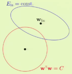
Choose a $\weight$ that lies on both of the ellipsoid boundaries. From here, we can visualize the gradient of $\insample$ with respect to the chosen point as well as the orthogonal vector to the red ellipsoid. The orthogonal vector to the red ellipsoid is equivalent to $\weight$ (from the center). From visualizing these vectors, we can tell that the chosen point below doesn’t minimize $\insample$. If it did minimize $\insample$, then both vectors would be directly opposite each other:

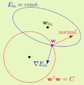
A condition can therefore be expressed that the gradient of the solution $\weightreg$ when found should be proportional to the negation of $\weightreg$:

The solution of the last equation is simply the minimization of the following:

The values of $C$ and $\lambda$ are related, so that if $C$ is so big it already contains $\weightlin$, so $\lambda$ can be thought of as being $0$, and corresponding to the simple minimization of $\insample$. When $C$ is smaller, $\lambda$ has to go up:

Augmented Error

We’re now going to consider an augmented error $\def \augerror {E_{\text {aug}}} \augerror$ that is essentially $\insample$ augmented with the regularization term:

The key observation is that solving the above equation is equivalent to minimizing $\insample$ subject to the constraint $\weightT \weight \leq C$. This constraint lends itself to VC analysis.

To minimize this, we take the gradient of $\augerror$ and equate it to $\mathbf 0$:

So now this results in the weight vector with regularization, $\weightreg$:

This is opposed to the weight vector without regularization, $\weightlin$, which can be achieved by simply setting $\lambda = 0$:

We can now observe the effects of varying $\lambda$. In the first example, there is apparent overfitting. However, as $\lambda$ increased, there is apparent underfitting. Clearly, the choice of $\lambda$ is important:

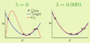
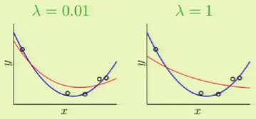
Weight Decay

The name of the regularizer that involves minimizing the following quantity is referred to as weight ‘decay’:

For example, in batch gradient descent, we take a step from $\weight(t)$ to $\weight(t + 1)$:

This can be interpreted geometrically. In the usual implementation of batch gradient descent we have the previous step $\weight(t)$ that is moved in the direction of the gradient $\nabla \insample$. However, this now includes a regularization term which can be interpreted as a nudge factor. That is, it takes the previous position, nudges it a bit based on $\lambda$, and then performs the gradient descent. This is why the regularizer is called weight decay, because the weights decay from one iteration to the next.

In neural networks, the term $\weightT \weight$ can be computed by considering all of the weights in all of the layers, input units, and output units and squaring them and summing them up:

Variations of Weight Decay

Instead of having a fixed budget $C$ and having the sum of the squared weights being less than or equal to $C$, we could emphasize certain weights by using this regularizer:

Here, $\gamma$ is referred to as the importance factor. For example, if a particular $\gamma_q$ is small then the equivalent weight $w_q$ is less restricted; it can be made larger while knowing it won’t take up too much of the budget $C$. On the other hand, if a particular $\gamma_q$ is big, then the corresponding weight doesn’t have that luxury.

For example, imagine that $\gamma_q$ is set to $2^q$. In this case, the regularizer is giving a larger emphasis on higher order terms. What this means is that the regularizer is trying to find a low-order fit. For example, a 10th-order polynomial would quickly kill the budget because $\gamma_{10} = 2^{10}$. If instead we had $\gamma_q$ set to $2^{-q}$, it would look for a high-order fit.

In neural networks, the importance factor $\gamma$ is given different values for each each layer, in other words, giving different emphasis for the weights in different layers.

The most general regularizer is called the Tikhonov regularizer, which has the form:

This is a general quadratic in matrix form. Weight decay, low-order fits, high-order fits, and many other regularizations can be achieved given the proper choice of matrix $\mathbf \Gamma$.

Weight Growth

Just as big weights were constrained earlier, small weights can also be constrained. The following shows a plot of weight decay’s $\outsample$ as a function of the regularization parameter $\lambda$. Notice that it dips before it goes back up again, in which case it begins to underfit. This means that weight decay performs well given the correct choice of $\lambda$. Weight growth on the other hand—constraining weights to be large—is considerably worse.

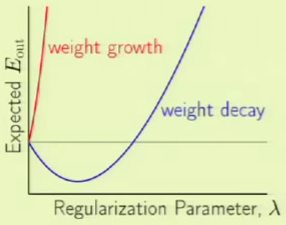
Stochastic noise is “high-frequency”. Deterministic noise is also non-smooth. Because of these common observations, the guideline is to constrain learning towards smoother hypotheses. This is because the regularizer is a cure for fitting the noise. For this reason, we want to punish the noise more than we are punishing the signal. The usual way that hypothesis sets are mathematically written as a parameterized set is by having smaller weights correspond to smoother hypotheses.

Generalized Regularizer

The regularizer will be referred to as $\Omega$:

We will minimize the augmented error of the hypothesis:

This looks similar to the VC dimension:

From this, we make the claim that $\augerror$ is better than $\insample$ as a proxy of $\outsample$.

The perfect regularizer is one that restricts in the “direction” of the target function. Regularization generically applies a methodology which harms the overfitting (fitting the noise) more than it harms the fitting (fitting the guideline), therefore it’s a heuristic. For this reason, we move in the direction of smoother or “simpler” because the noise itself is not smooth. For example, in the case of movie ratings, this kind of regularization guideline tends to opt for the average rating in the absence of enough examples.

If we choose a bad regularizer $\Omega$, we still have $\lambda$ that can save us by means of validation, which can set $\lambda$ such that it completely ignores the bad regularizer $\Omega$. In any case, having a regularizer is necessary to avoid overfitting.

Neural Network Regularizers

Remember that the $\tanh$ function acts linear for small value ranges and binary for larger value ranges.

Neural Network Weight Decay

If we use small weights, then the signal is constrained to the range that produces linear-like values, so every neuron would essentially be computing the linear function. With multiple hidden layers in a neural network, this essentially becomes a complex neural network that is computing a very simple linear function.

If weights are increased to the maximum, $\tanh$ outputs binary values, which results in a logical dependency that can be used to implement any kind of functionality.

Given these two extremes, it’s apparent that as weights are increased, the model produces more complex models. This represents a clear correspondence between the simplicity of the function being implemented and the size of the weights, which is properly represented by weight decay.

Neural Network Weight Elimination

Weight elimination works by remembering that the VC dimension of neural networks is more or less the number of weights, so it simply eliminates some of the weights by forcing them to be $0$, so that the number of free parameters decreases, as does the VC dimension, leading to a better chance of generalizing and less chance of overfitting.

Determining which weights to eliminate can is a combinatorial problem. Soft weight elimination is an optimization of weight elimination. For very small weights, regular weight decay is applied. For very large weights, the result is close to $1$. In other words, big weights are left alone and small weights are pushed towards $0$, or “soft eliminated”:

Early Stopping in Neural Networks

Recall that early stopping consists of stopping before $\outsample$ begins to increase. This is regularization through the optimizer. The point at which to stop is determined through validation.

Optimal $\lambda$

Observing the optimal value of $\lambda$ given the different levels of noise provides some insight as to how deterministic noise is treated by the regularizer compared to how it treats stochastic noise.

As the level of stochastic noise $\sigma^2$ increases, the level of regularization $\lambda$ necessary to achieve the minimum $\outsample$ increases. For example, when there is no noise, the minimum $\outsample$ can be achieved with $\lambda = 0$. However, as the noise increases, regularization is necessary to achieve the best possible $\outsample$. The left side of the red and green curves represent the overfitting that occurs without regularization.

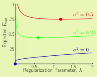
The same behavior is observed as the level of deterministic noise $Q_f$ (complexity of the target function) increases.

This cements the correspondence that regularization behaves with respect to deterministic noise behaves almost exactly as if it were unknown stochastic noise.

Validation

Remember that regularization tried to estimate the “overfit penalty;” so that instead of minimizing just $\insample$ it would minimize $\insample$ plus the overfit penalty, a quantity known as the augmented error $\augerror$. Validation instead tries to estimate the actual $\outsample$ and tries to minimize it directly.

To arrive at this estimate, we first find an out-of-sample point $(\weight, y)$, that is, a point that was not involved in training, otherwise known as a validation point. The error for this point is $\crossentropy(h(\weight), y)$. The error itself could be the squared error, binary error, etc., and we consider it to be an estimate of $\outsample$, which we can do because:

This is an unbiased estimate of $\outsample$. The variance is known as $\sigma^2$:

The variance of estimating $\outsample$ from a single point would be very high, so instead of calculating this estimate from a single point, we do it from an entire validation set $(\weight_1, y_1), \dots, (\weight_K, y_K)$. Notice that the total number of points in the validation set is $K$, as opposed to $N$ in the training set. The validation error derived from this validation set is known as $\def \valerror {E_{\text {val}}} \valerror$:

Therefore the expected value of $\valerror$ is:

The variance is computed as:

The validation error:

Given the data set $\mathcal D = (\weight_1, y_1), \dots, (\weight_N, y_N)$, take $K$ points at random and use them for validation, which leaves $N - K$ for training. The set of $N - K$ training points is called $\def \trainingset {\mathcal D_{\text {train}}}$ and the set of $K$ validation points is called $\def \validationset {\mathcal D_{\text {val}}}$.

We established that the reliability of the estimate of the validation set is of the order $\smash {\frac 1 {\sqrt K}}$, so the smaller the size $K$ of the validation set, the worse off the estimate is. On the other hand, if we use a very large $K$ we would get a reliable estimate of a worse quantity of $\outsample$, because the $\outsample$ decreases with the increase in training set size, the size of which must decrease if we increase the validation set size.

We would instead like to estimate the error using the validation set, then once we have the estimate, return the $K$ points to the training set. We begin by deciding that the data set $\mathcal D$ is comprised of $\trainingset \cup \validationset$. Previously when we used the entire training set $\mathcal D$ we arrived at the final hypothesis $g$. However, when using only $\trainingset$, we will call the resulting final hypothesis $g^-$ to remind ourselves that it’s not based on the full training set.

$\trainingset$ yields $g^-$ which is then evaluated on $\validationset$ in order to get the estimate $\valerror(g^-)$. Then the final hypothesis $g$ is derived using the full set $\mathcal D$. This means that there will be a discrepancy between the estimate $\valerror(g^-)$ and $\valerror(g)$, because they are based on different hypotheses, as derived from different training sets. This presents a trade off between the size of $\trainingset$ and $\validationset$: a larger $\trainingset$ means that the hypothesis more closely resembles the final hypothesis, but a subsequently smaller $\validationset$ makes the estimate a poor one, even if the hypothesis $g^-$ is representative of the final hypothesis $g$.

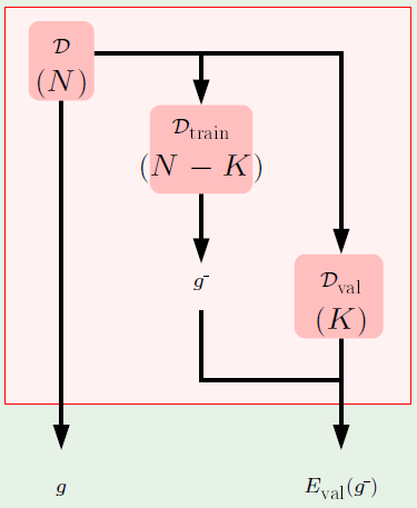
The rule of thumb for the choice of the size $K$ of $\validationset$ is to make it $1/4^{\text {th}}$ the size of of the full set $\mathcal D$:

Purpose of Validation

Looking back at the early stopping curve, if we used $K$ points to estimate $\outsample$ then the estimate would be called $E_{\text {test}}$ if we don’t perform any actions based on this estimate. As soon as we decide to perform an action based on it, such as stopping, then the previous $\insample$ is considered the validation error, because it is now considered to be biased. The difference is that the test set is unbiased, whereas the validation set has an optimistic bias.

For example, given two hypotheses $h_1$ and $h_2$ with $\outsample(h_1) = \outsample(h_2) = 0.5$ and error estimates $\crossentropy_1$ and $\crossentropy_2$ that are uniform on $[0,1]$. Now pick $h \in \{h_1, h_2\}$ based on $\crossentropy = \min(\crossentropy_1, \crossentropy_2)$. The value of $\mathbb E(\crossentropy) < 0.5$, because given two variables, the probability that one of them is $< 0.5$ is $75\%$, since the probability that both them are $0.5$ is $0.5 * 0.5 = 25\%$. This means that $\mathbb E(\crossentropy)$ is an optimistic bias. This bias has a negligible effect on overall learning.

Model Selection

The main use of validation sets is model selection, which is accomplished by using $\validationset$ more than once. We begin with $M$ models $\mathcal {H_1, \dots, H_M}$ to choose from. This could be models such as linear models, neural networks, support vector machines, etc. It could also be that we’re only using polynomial models, in which case the question is whether to use 2nd, 3rd, 4th-order etc. It could also be that we’re only using 5th-order polynomials, in which case the question is the value of $\lambda$ being for example $0.01, 0.1$ or $1.0$. All of this falls under model selection, based on $\outsample$ by means of $\validationset$.

Then we will use $\trainingset$ to learn $g_m^-$ for each model. The hypothesis $g_m^-$ is then evaluated using $\validationset$ to derive $E_{\text m}$, which is simply $\valerror(g_m^-)$. The model with the smallest $E_{\text m}$ is chosen as the optimal model $m^*$, which is then used to train on the entire dataset $\mathcal D$ to derive the hypothesis $g_{m^*}$.

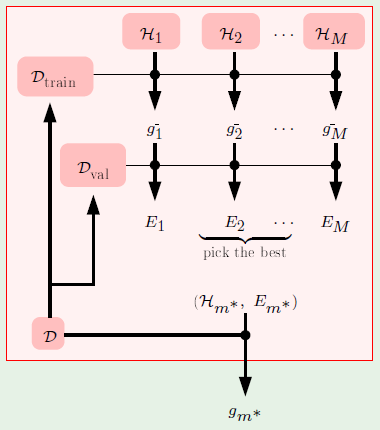
Validation Bias

The bias is introduced because we chose the model $\mathcal H_{m^*}$ using $\validationset$, so $\valerror(g_{m^*}^-)$ is a biased estimate of $\outsample(g_{m^*}^-)$. The following graph depicts two models to choose between, one being 2nd-order and the other 5th-order polynomials. It’s not shown which model was chosen.

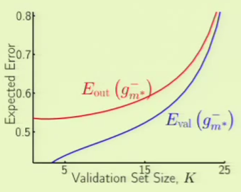
The curve for $\valerror$ goes up because the higher the $K$, the less points that are left for $\trainingset$. The curve for $\outsample$ goes up because it is based on the number of points left in $\trainingset$, so the error increases as there are less and less points.

The curve for $\valerror$ converges with $\outsample$ because $K$ is increasing, which means that the estimate $\valerror$ is more and more accurate.

It can be considered that $\validationset$ is actually used for “training” on a very special kind of hypothesis set, known as the finalists model, which consists of the hypotheses derived from each model:

Now when we measure the bias between $\valerror$ and $\outsample$, where $\valerror$ can be thought of as the training error of this special set $\mathcal H_{\text {val}}$. This means we can go back to Hoeffding and VC, to say that:

If for example we’re trying to determine the value of $\lambda$, it can be thought of as being able to take on an infinite number of values, however, instead it can be though of as being a single parameter, which according to the VC inequality is not a problem. This applies to regularization which is trying to determine the value for the single parameter $\lambda$, or early-stopping which is trying to determine the value for the single parameter $T$ (number of epochs to perform). In both cases, they more or less correspond to having one degree of freedom.

Data Contamination

The error estimates encountered so far have been $\insample$, $E_{\text {test}}$, and $\valerror$. These can be described as data contaminations, where if the data is used to make choices, it is being contaminated as far as its ability to estimate the real performance. In this sense, contamination is the optimistic (deceptive) bias in estimating $\outsample$.

The training set is totally contaminated. For example, if it’s put through a neural network with 70 parameters that yielded a very low $\insample$, we can be assured that $\insample$ is no indication of $\outsample$, in which case $\insample$ can’t be relied upon as an estimate for $\outsample$.

The validation set is slightly contaminated because it made a few choices.

The test set, on the other hand, is completely clean, since it wasn’t used in any decisions, so it is unbiased.

Cross-Validation

We would like to know the actual $\outsample(g)$, but we only have $\valerror(g^-)$, which is supposed to be an estimate for $\outsample(g^-)$. Therefore it is necessary for $K$ to be small so that $g^-$ is fairly close to $g$, since the bigger $K$ is, the larger the discrepancy between the training set and the full set, and therefore larger the discrepancy between $g^-$ and $g$. This creates a dilemma because we would like $K$ to be large, to increase the reliability of $\valerror(g^-)$ as an estimate for $\outsample(g^-)$.

It’s possible to achieve both constraints by using a technique called leave one out. First choose $N - 1$ points for training and $1$ point for validation. The training set $\mathcal D_n$ is denoted by the point that was $n$ that was left out:

The final hypothesis learned from $\mathcal D_n$ is called $g_n^-$, since it was trained on all examples except $n$. The validation error is then defined as simply the error on the left-out point using the hypothesis derived from the set that excludes that point. We can be sure that this estimate is an unbiased estimate, albeit a bad estimate:

This can then be repeated for every point in the data set using every $\mathcal D_n$. What is common between every error measure is that it was computed using the hypothesis derived using a training set of $N - 1$ points, albeit different points.

The cross validation error is then defined as:

The effective size of the validation set represented by the cross validation error is very close to $N$.

For example, given three points, we train three different sets:

The cross validation error can then be defined as:

This cross validation error can then be interpreted as how well the linear model fits the data out of sample.

Cross-validation can then be used for model selection. Compare the above linear model example with the constant model:

In this case, the constant model is clearly better.

Going back to the case of hand-written digits classification, where we extracted two features: symmetry and intensity. We will sample 500 points for training and the rest for testing the hypothesis. The non-linear transformation is 5th-order:

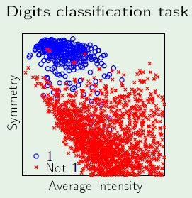
In this case, we would like to use cross-validation to determine at which point to cut off the non-linear transformation, that is how many terms to use, where each term in the non-linear transformation is considered a separate model, for a total of $20$ different models. Here are the different errors derived based on the number of features used:

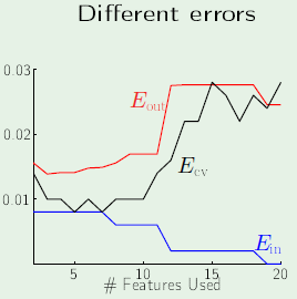
From this graph it seems that the best number of features to use is 6. Without validation (left) we can observe overfitting with no in-sample error and $2.5\%$ out-of sample error, whereas with validation (right) provides a smooth surface with non-zero in-sample error but lower out-of-sample error at $1.5\%$.

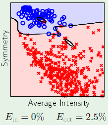
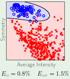
Cross-Validation Optimization

When we use leave one out, we have $N$ training sessions on $N - 1$ points each. We would like to use more points for validation. We take the data and break it into different folds, such as 10 folds, making it 10-fold cross-validation. We use one fold for validation and the other 9 for training. In other words, it’s similar to leave one out except instead of leaving one point out we leave out a chunk/fold.

This results in $\frac N K$ training sessions on $N - K$ points each. Specifically, 10-fold cross validation is very useful in practice.

Support Vector Machines

Going back to the concept of dichotomies, when we wanted to determine the number of ways in which a model could separate data in different configurations. With the linear model, we ignored the actual position and angle of the line that separated the data, only caring for different resultant configurations.

However, if we did care about the position and angle of the line, it could be said that a distinguishing factor of every such line position and angle would be its margin of error, that is, its distance between the data it separates. A higher margin of error makes it more tolerant to out-of-sample data, due to noise for example. We can enforce a lower bound requirement on the margin of error, which naturally would result in less dichotomies, as it places a restriction on the growth function, yielding a smaller VC dimension:

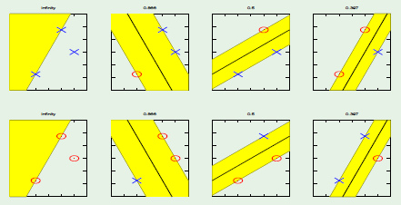
In the scenario in which we would like to enforce a lower bound on the margin of error, the problem of learning then becomes that of finding the $\weight$ that maximizes the margin.

To find the $\weight$ with a large margin we first pick $\feature_n$ that is the nearest data point to the hyperplane $\weightT \feature = 0$. We would like to determine the distance between the point and this hyperplane, which would represent the margin.

First we normalize $\weight$ with the following constraint, where $\feature_n$ again represents the nearest point to the hyperplane:

Second we have to take out $w_0$, the threshold/bias weight, from now on referred to as $b$:

Now the hyperplane is defined as follows, with $x_0$ absent since it was always $1$ and $w_0$ was taken out as $b$:

We can now compute the distance between $\feature_n$ and the plane $\weightT \feature + b = 0$ where $|\weightT \feature_n + b| = 1$. First we must realize that the vector $\weight$ is perpendicular to the plane in $\mathcal X$-space. For example, pick any $\feature'$ and $\feature''$ on the plane. Since they’re on the plane, they must satisfy the plane equation so that:

The conclusion from the above is that $\weight$ is orthogonal to any vector on the plane.

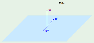
The distance between the nearest point $\feature_n$ and the plane can be computed by taking any point $\feature$ on the plane and computing the projection of the vector formed by $\feature_n - \feature$ on $\weight$. In order to get this projection, we need the unit vector of $\weight$:

So that now the distance can be computed as:

The last component of the penultimate equation disappears because the equation for a point on the plane is defined to be $0$, and we already restricted the equation for $\feature_n$ to be equal to $1$.

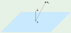
The resulting optimization problem is to maximize the margin, denoted as $\smash {\frac 1 {\lVert \weight \rVert}}$ subject to the following constraint:

However, this is not a friendly optimization problem because it has a $\min$ in it. To get rid of the absolute value, notice that:

Now instead of maximizing $\smash {\frac 1 {\lVert \weight \rVert}}$ we will minimize the following quantity:

The domain of this optimization problem is $\weight \in \mathbb R^d, b \in \mathbb R$. This is therefore a constrained optimization problem, for which we can use Lagrange, but the problem is that these are inequality constraints not equality constraints.

We saw this scenario before with regularization, where we minimized $\insample(\weight)$ under a constraint:

We found that $\nabla \insample$ was normal to the constraint. This presents a conceptual dichotomy between regularization and SVM. In regularization, we optimize the in-sample error $\insample$ under the constraint $\weightT \weight$. Conversely, with SVM we are optimizing $\weightT \weight$ under the constraint that $\insample = 0$.

method	optimize	constraint
Regularization	$\insample$	$\weightT \weight$
SVM	$\weightT \weight$	$\insample$

Lagrange Formulation

To recap, we are performing the following constrained optimization:

We first take the inequality constraint and put it in zero-form, so that:

This is then combined with the optimization component to form the full optimization problem, which is a Lagrangian $\mathcal L$ dependent on $\weight$, $b$, and the Lagrange multipliers $\alpha$:

Now we can find the gradient of the Lagrangian with respect to the weight, which we want to minimize by setting it to the zero-vector:

Now we find the derivative of the Lagrangian with respect to $b$ in order to minimize it by setting it to zero:

We now want to combine these optimization components in order to remove the $\weight$ and $b$ from the optimization problem, so that it’s instead only a function of $\alpha$. This is referred to as the dual formulation of the problem:

We still have to get rid of the constraints in order to have a pure optimization problem that we can pass on to some external quadratic programming library. First of all, most quadratic programming packages perform minimizations not maximizations, so we have to convert it to a minimization, which is accomplished by simply negating the equation:

Next we want to isolate the coefficients from the $\mathbf \alpha$ values, since the $\mathbf \alpha$ are parameters. What the quadratic programming library receives are the coefficients of our particular problem $y$ and $\feature$ and produces the $\mathbf \alpha$ values that minimize the above equation. This is accomplished as follows:

The matrix in this equation as well as the linear coefficients are passed to the quadratic programming library. The above equation is equivalent to:

It’s important to note the implications of the number of examples, which clearly yields a larger matrix, in which case there are a variety of heuristics that mitigate this problem.

After being fed the quadratic and linear coefficients, the quadratic programming library produces the vector $\mathbf {\alpha} = \alpha_1, \dots, \alpha_N$, from which we need to determine the value of $\weight$, $b$, the margin, and so on. The weights can be computed as based on the previous constraint that concerned it:

It might be surprising to realize that the majority of the $\mathbf \alpha$ vector consists of zero elements (interior points). This is due to a Karush-Kuhn-Tucker (KKT) condition that’s relevant here that says that either the slack is zero or the Lagrange multiplier is zero, such that their product is definitely zero:

We saw this before in regularization, where we had a constraint which was to be within the red circle while optimizing a function represented by the blue circle. When the constraint didn’t really constraint us and the absolute optimal was within the blue circle, there was no need for regularization and so $\lambda = 0$.

The points which define the plane and margin are the ones for which the $\alpha$ values are positive, and all of these values form a support vector:

That is, we had $N$ points which we classified and for which we found the maximum margin, and the margin touched some of the $+1$ and some of the $-1$ points, and it is said that these points “support the plane,” and are called support vectors, while the rest of the points are interior points. In the image below, the support vectors are those points that touch the extents of the margin, those with a circle around them:

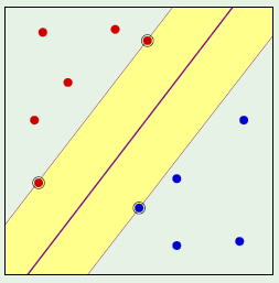
Since most $\alpha$ are zero, the weight calculation can be changed to only sum those in the support vector:

We can also solve for the bias $b$ corresponding to threshold term using any support vector, for which we already know that:

SVM Non-Linear Transformations

Although all of this so far has only handled situations where the data is linearly separable, it’s possible to attempt to solve it using non-linear transformations in the $\mathcal Z$-space as we did with perceptrons.

Observing the equation to maximize, we can see that there are only two components which may need to change in this transition between the $\mathcal X$-space and the $\mathcal Z$-space.

The increase in dimensionality resulting from the non-linear transformation has no effect on the complexity of the optimization. The quadratic optimization process results in the $\alpha$ vector, which is interpreted in the original $\mathcal X$-space.

During a non-linear transformation, the support vectors resulting from the optimization “live” in $\mathcal Z$-space. In $\mathcal X$-space, these same points can be thought of as “pre-images” of support vectors, those with a circle around them:

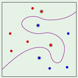
It’s important to remember that the distance between the points in $\mathcal X$-space and the resulting curve are not the margin, since the margin is maintained only in $\mathcal Z$-space.

What’s interesting is that even if the non-linear transformation involved a million-dimensional transformation, we ended up with four support vectors, which effectively corresponds to having four parameters, so that generalization applies to the four parameters and not the entire million. This means we’re able to use the flexibility of a higher dimensional representation without sacrificing generalization. In other words, we have a complex hypothesis $h$, but a simple hypothesis set $\mathcal H$. Therefore, the generalization result is:

Kernel Methods

We want to go to the $\mathcal Z$-space without paying the price for it. We saw previously that going to the $\mathcal Z$-space involved a very simple dot product:

We would like to see if we could do away with this relatively low cost altogether. The constraints for this equation are:

Notice that $\mathbf z$ isn’t present in the constraints. The hypothesis is essentially:

We can then substitute the weight’s definition into the hypothesis function, in which case we require the inner products consisting of $\mathbf z_n^\intercal \mathbf z$. We can do the same exact thing to determine the value of $b$, in which case we need $\mathbf z_n^\intercal \mathbf z_m$. In effect, this means that we only deal with $\mathbf z$ as far as the inner product in the hypothesis function is concerned.

Kernel Trick

Polynomial Kernel

Given two points $\feature$ and $\feature' \in \mathcal X$, we need $\mathbf z^\intercal \mathbf z'$. Let $\mathbf z^\intercal \mathbf z' = K(\feature, \feature')$, where $K$ is referred to as the kernel, which corresponds to some $\mathcal Z$-space, it is considered the “inner product” of $\feature$ and $\feature'$ after some transormation. For example $\feature = (x_1, x_2)$ undergoes a 2nd-order non-linear transformation:

So the kernel would be defined as:

Now the question is whether or not we can transform the kernel $K(\feature, \feature')$ without transforming $\feature$ and $\feature'$ into the $\mathcal Z$-space. Consider the following:

This looks very similar to an inner product if it weren’t for the twos, in which case it’d be as if we transformed to the 2nd-order polynomial and took the inner product there. However, this is an inner product if we say that the transformation that we are using is:

The advantage of the kernel is that we don’t have to take each feature and expand it per the non-linear transformation in order to perform the inner product, instead we directly compute the inner product from the $\mathcal X$-space feature vector.

More specifically, this is called the polynomial kernel. Generally, given a general d-dimensional space $\mathcal X = \mathbb R^d$ with a transformation of that space into a Qth-order polynomial $\Phi\colon \mathcal {X \to Z}$, the “equivalent” kernel would be:

A kernel of the above form corresponds to an inner product in a higher space. So now all we have to do is use the $\mathcal X$-space feature vectors, compute the dot product, and raise that value to some exponent, instead of having to explicitly go into the $\mathcal Z$-space. This is all guaranteed if the kernel $K(\feature, \feature')$ is an inner product in some space $\mathcal Z$-space. Consider the following kernel:

This kernel is clearly a function of $\feature$ and $\feature'$. It doesn’t have a clear inner product. Does this correspond to an inner product in $\mathcal Z$-space? Indeed it is, if the $\mathcal Z$-space is treated as being infinite-dimensional. In this case we would get the full benefit of a non-linear transformation, without worrying about the generalization ramifications of going to an infinite-dimensional space. For example, take a simple case where the kernel is applied to a one-dimensional $\mathcal X$-space and $\gamma = 1$:

The $x$ terms can be grouped together and so can the $x'$ terms, and ultimately this equation can be transformed to look like an inner product in an infinite space, due to the infinite summation. This kernel is called the radial basis function (RBF) kernel.

To see it in action, in the case of a slightly non-separable case in the $\mathcal X$-space with a slightly curvy target function. We transform this dataset into an $\infty$-dimensional $\mathcal Z$-space. The red and blue points are the support vectors (9 total; 4 blue, 5 red), the lime curve is the target function and the black curve is the $\mathcal Z$-space hyperplane:

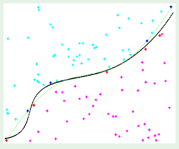
Here we were able to visit an infinite-dimensional space and yield only 9 support vectors, which thanks to the error bound we developed earlier means that the out-of-sample error must be less than about $10\%$. Previously, going to an infinite or even higher order $\mathcal Z$-space was considered overkill, but that determination is now made based on the number of resultant support vectors.

An important thing to remember is that the distances between the support vectors and the $\mathcal X$-space hyperplane will possibly not be minimal, because that distance that was solved for was solved in $\mathcal Z$-space not $\mathcal X$-space. The support vectors are not support vectors per se, but rather they are “pre-images” of the actual support vectors in the $\mathcal Z$-space.

Kernel Formulation of SVM

In solving support vector machines, we would pass the inner products of the feature vectors to the quadratic programming library. All that changes now is that we instead pass the result of the kernel function $K$; everything else remains the same:

When we receive the $\alpha$ and we need to construct the hypothesis in terms of the kernel. In other words, we want to express $g(\feature) = \sign(\weightT \mathbf z + b)$ in terms of $K(-, -)$. First remember the definition of the weight:

So now we can construct the hypothesis, which is also the general SVM model, which differs based on the kernel function:

Kernel Function Validity

How can we determine that a kernel is valid, i.e. that it corresponds to an inner product in some space, without visiting that space? In other words, how do we know that $\mathcal Z$ exists for a given $K(\feature, \feature')$?

There are three approaches to come up with a valid kernel. The first method is by construction. The second is by using mathematical properties of the kernel (i.e. Mercer’s condition), which have already been applied to kernel functions other people have developed which can be applied to our own problems. The third approach is to simply not care whether or not $\mathcal Z$ exists, which is an approach taken by a number of people but for which Professor Yaser Abu-Mostafa has reservations, since the guarantees of the method depend on $\mathcal Z$ existing.

To take the second approach for the purposes of designing our own kernel. A kernel $K(\feature, \feature')$ is a valid kernel iff:

1. It is symmetric so that $K(\feature, \feature') = K(\feature', \feature)$
2. The matrix of all possible pairs of feature vectors applied to the kernel function is positive semi-definite, that is, the matrix should be greater than or equal to 0, for any $\feature_1, \dots, \feature_N$. This is known as Mercer’s condition:

Soft-Margin SVM

There are two main kinds of non-separable situations. Slightly non-separable (left) is when it might be beneficial to simply accept that as error using something like the pocket algorithm, as opposed to sacrificing generalization in order to capture what are potentially simply outliers. Seriously non-separable (right) is when it’s not a matter of outliers, but that the data is simply non-linearly separable.

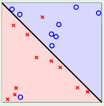
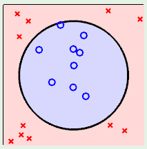
Slightly-separable data can be handled by soft-margin SVM, while seriously non-separable data can be handled by kernel functions. In real world data sets, however, it’s likely that there will be elements of both: built-in non-linearity with outliers. For this reason, we would be combining kernels with soft-margin SVMs in almost all of the problems that we would encounter.

Soft-Margin SVM Error Measure

The error measure will be defined by a so-called margin violation, which could be the point within the margin in the image below. Even though it is correctly classified by the hyperplane, it’s considered a margin violation because it falls within the margin.

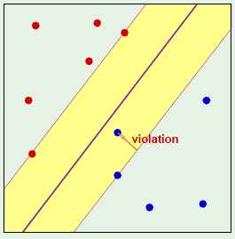
It can be said that the margin is violated when $y_n(\weightT \feature_n + b) \geq 1$ fails. This failure can be quantified by introducing a “slack” $\xi_n \geq 0$ for every point so that:

The total violation made by a derived SVM can be expressed as the sum of the slacks, since those that don’t violate the margin will have $\xi = 0$:

Soft-Margin SVM Optimization

The previous optimization that we performed was to minimize the following quantity, which had the effect of maximizing the margin:

Now we are going to add an error term that corresponds to the violation of the margin:

In this new optimization problem, $C$ is a constant that represents the relative importance of the error versus the margin, similar to augmented error. For example, a very high value of $C$ represents that error cannot be afforded, whereas a very low value of $C$ means that we can have a large margin but it would have a higher rate of errors.

The Lagrange formulation for this optimization problem can thus be derived as follows, where the first equation is the original Lagrange formulation:

The minimization with respect to $\weight$ is the same as before:

The minimization with respect to $b$ is also the same as before:

The minimization with respect to $\xi$ can be derived as follows:

The ramifications of the final equation is that the Lagrange formulation above reduces back down to the original Lagrange formulation, with the only added constraint that $\alpha_n$ be at most $C$:

The result of this minimization is the weight:

This particular weight guarantees that we are minimizing the quantity:

In practical terms, well we have to do to use a soft-margin is to ensure that $0 \leq \alpha_n \leq C$.

Types of Support Vectors

We call the support vectors that fall on the hyperplane boundary margin support vectors ($0 \lt \alpha_n \lt C$):

The other vectors that don’t fall on the hyperplane boundary but are still correctly classified are referred to as non-margin support vectors ($\alpha_n = C$):

The $C$ parameter is determined in practice using cross-validation.

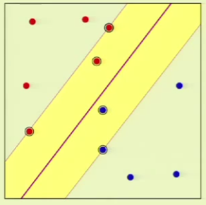
There are two final observations.

First, with the hard margin, what happens if the data is not linearly separable? The translation from the “primal” form (minimizing $\weightT \weight$) to the “dual” form (maximizing $\mathcal L(\alpha)$) begins to break down. This is mathematically valid only if there is a feasible solution. The point is that we don’t have to worry about this, we don’t have to go through the combinatorial process of determining whether a data set is linearly separable. Instead, we can validate the solution.

Second, when we transform to the $\mathcal Z$-space, some of these transformations had a constant coordinate of $1$. This used to correspond to $w_0$, but we made a point to state that in support vectors there are no $w_0$ values, since we took them out as a separate variable $b$. If the $\mathcal Z$-space transformation has a $w_0 = 1$, then we effectively have two variables doing the same thing. We don’t have to worry about this either though because when we get the solution, all of the corresponding weights will go to $0$, and the bulk of the bias will go to $b$.

Radial Basis Functions

Radial basis functions serve as the glue between many different machine learning topics. The idea is that every point in the data set $(\feature_n, y_n) \in \mathcal D$ influences the value of the hypothesis $h(\feature)$ at every point $\feature$ based on the distance to nearby points $\lVert \feature - \feature_n \rVert$. For example, imagine in the bottom image that the top of the bump is $\feature_n$ and the surface represents the influence to other points, and the symmetry of the function shows that this influence is a function of the distance.

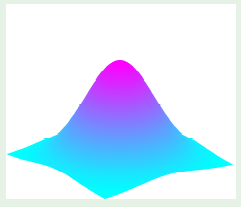
The standard form of of a radial basis function embeds the notion that the closer a point is to the feature point, the more of an influence it has on it:

The equation shows the source of the basis function part of the name, while the radial part of the name comes from the $\lVert \feature - \feature_n \rVert$.

Now that we have the model, we can move on to the learning algorithm, where we want to find the parameters $w_1, \dots, w_n$. First it’s useful to note that we have $N$ parameters $w_n$, so it shouldn’t be difficult to find parameters such that $\insample = 0$, so that $h(\feature_n) = y_n$ for $n = 1, \dots, N$. This constraint can be expressed as follows:

This shows that there are $N$ equations, one for each data point with $N$ unknown $w$ parameters.

If $\mathbf \Phi$ is invertible, then the solution is simply:

This solution can be interpreted as being an exact interpolation, because on the points for which we know the value of the hypothesis, we’re getting the exact output $y$ value.

Effect of $\gamma$

The effect of $\gamma$ is such that if it is small, the Gaussian is a wider curve, whereas if it were larger it’d be a steeper curve. Depending on where the points are—specifically how sparse they are—the steepness of the curve makes a difference.

The image on the left shows the effect of choosing a small $\gamma$. The three training points are on the curve, since that was what the constraint was. The smaller gray curves are the individual contributions from each of the points, that is, $w_1, w_2, w_3$, such that when they’re plugged into the hypothesis function it yields the blue curve.

The image on the right shows the effect of choosing a larger $\gamma$. The interpolation between any two points is poor because the individual contributions of each point “dies out” too quickly.

It’s apparent that $\gamma$ has an effect on the performance of interpolation, and that it seems to depend on the data set in question, specifically, how far apart the points are. We will cover the choice of $\gamma$ later on.

RBF Classification

The model described above was a regression model, where we considered the output to be real-valued which was matched with the target output which was also real-valued. It’s possible to use RBFs for classification, however, by modifying the hypothesis function to be:

The question now is how to determine the $w_n$ values with this $\sign$ function now involved. We’ve done this before when we applied linear regression for classification. We will focus on the inner component of the $\sign$ function, the signal $s$:

Where we will try to make the signal itself match the $\pm 1$ target. So that we can minimize $(s - y)^2$ on $\mathcal D$ knowing that $y = \pm 1$, then we simply return $h(\feature) = \sign(s)$.

RBFs share a relationship to the nearest-neighbor method, where we classify by looking at the closest point $\feature_n$ within the training set to the point $\feature$ being considered, so that $\feature$ inherits the label $y_n$ corresponding to that closest point $\feature_n$. For example in the image below, all points in a given red-shaded region inherit the label of the red point within that region because all points within that region are closest to that point rather than any of the other points that define other different regions:

This can be approximated with RBFs, where we only take influence of nearby points. The basis function would look like a cylinder as in the image below, where it’s a given constant value or zero. With this basis function, the regions would look more like the cylinders.

The nearest-neighbor approach is pretty brittle, as the boundaries between the regions are abrupt. It can be modified into the $k$-nearest neighbors, where instead of taking the value of the closest point, we look at the $k$ nearest points and adopt the label most represented by those points. This has an effect of smoothing the surface, where the number of fluctuations will decrease.

The RBF can be smoothed similarly by using a Gaussian instead of a cylinder, which does a good job of representing a gradual decrease in influence.

In both cases, the model can be considered as a similarity-based method, where we are classifying points according to how similar they are to points in the training set.

K-Centers RBF

We are generally mindful of generalization as a ratio between the number of parameters and data points. However, the RBF model we described has $N$ parameters $w_1, \dots, w_N$ based on $N$ data points, so it may seem hopeless to generalize. We can mitigate this by preventing every point from having its own influence, and instead appoint a number $K$ of important centers for the data and have them influence the points around them.

We do this by taking $K \ll N$ centers $\mathbf {\mu_1, \dots, \mu_K}$ as the centers of the RBFs instead of $\feature_1, \dots, \feature_N$. The $K$ centers live in the same space as $\feature$, but they are not necessarily data points—they could be elected data points from the data set, or they may be specially constructed points that we may deem representative of the data set. We then define the hypothesis function as:

This hypothesis function now reflects the fact that every point $\feature_n$ is being compared against every center $\mathbf \mu_k$. We now have to determine how to choose the centers $\mathbf \mu_k$ and the weights $w_k$.

K-Means Clustering

To choose the $K$ centers, we are going to choose the centers as representative of the data inputs, that is, a representative center will exist for every cluster of data points. Such representative centers would be achieved by minimizing the distance between $\feature_n$ and the closest center $\mathbf \mu_k$. This is called K-means clustering because the center of a cluster will end up being the mean of the points in that cluster.

We begin by splitting the data set $\feature_1, \dots, \feature_N$ into clusters $S_1, \dots, S_K$. Again, a good representative center $\mathbf \mu_k$ of a cluster $S_k$ would minimize the distance between the points in the cluster and itself, represented as the sum of the Euclidean MSE between the candidate center and each of the points in the cluster. The optimal cluster configuration is achieved by then minimizing the sum of each cluster’s error measure.

This is unsupervised learning, since it was performed without any reference to the label $y_n$. The problem is that this is NP-hard in general; it is intractable to get the absolute minimum. The problem being NP-hard didn’t discourage us before when we realized that finding the absolute minimum error in a neural network was NP-hard as well, in which case we developed a heuristic—gradient descent—which led to back-propagation and thus a decent local-minimum.

LLoyd’s Algorithm

We can develop an iterative algorithm to to solve K-means clustering, which works by fixing one of the parameters and attempting to minimize the other. First it fixes the particular membership of the clusters $\feature_n \in S_k$ and it tries to find the optimal centers. After finding these centers, it then fixes these centers and tries to find the optimal clustering for these centers. This is repeated until convergence:

When updating $\mathbf \mu_k$, we essentially take the mean of the points in the cluster: add them up and divide by the amount of points in the cluster. This would be a good representative if $S_k$ were the real cluster.

The $\mathbf \mu_k$ value is then frozen and we cluster the points based on it. For every point $\feature_n$ in the data set, we measure the distance to the new center and admit it to the cluster $S_k$ if this distance is smaller than the distance between this point $\feature_n$ and any of the other clusters $\mathbf \mu_l$.

It is apparent that both steps are minimizing the original quantity, and since there are only a finite number of points and a finite number of possible values for $\mathbf \mu_k$, it is guaranteed that we will converge, albeit to a local minimum, which is sensitive to the initial centers or clusters, just like neural networks converged to a local minimum dependent on the initial weights. The general way of choosing decent initial centers or clusters is to perform a number of runs with different centers or clusters and choosing the best one.

LLoyd’s algorithm can be visualized in the image below. The algorithm is fed the only the inputs of the data set, with the centers initialized so some pre-defined values (black dots), then the algorithm iterates and outputs the representative $\mathbf \mu_k$ centers.

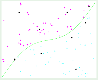
Notice that since we cluster values without looking at the label $y_n$, we can have clusters that lie on the boundary so that half of the points are $+1$ and the other half are $-1$. This is the price paid by unsupervised learning, where we want to find similarity as far as the input is concerned, not as far as the behavior with the target function is concerned:

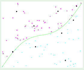
RBF Calculating Weights

Now that we have determined the centers we can determine the weights. Again the hypothesis function was defined as:

In this case there are now $N$ equations but only $K < N$ unknowns.

The weights can be solved for in the same manner as in linear regression by calculating the pseudo-inverse. If $\mathbf {\Phi^\intercal \Phi}$ is invertible, then:

In this case we aren’t guaranteed to get the correct value at every data point, but we do have a much higher chance at generalization since we only have $K \ll N$ parameters.

RBF Network

We can take the RBF model and design a graphical network in order to relate it to neural networks. In this graphical network, we take the input and compute the radial component, the distance to every $\center_k$. These radial components are handed to a non-linearity $\phi$, usually the Gaussian non-linearity. The resultant features are combined with weights $w_k$ in order to compute the output $h(\feature)$.

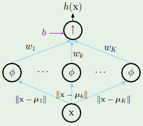
In this case the “features” are $\smash {\basis {\feature} {\center_k}}$. The non-linear transform features depend on $\mathcal D$, so it is no longer a linear model. However, since we only used the inputs in order to compute $\center$ it’s almost linear, since we didn’t have to back-propagate because we didn’t like the output, since the inputs were frozen. This is why the $w$ values look like multiplicative values, in which case it’s linear on those values.

A bias term ($b$ or $w_0$) is often added at the final layer.

RBF vs. Neural Networks

A two-layer neural network can be compared to an RBF network.

Both networks compute features, however in the case of RBF networks, the features depend on the distance to the center, and if that distance is very large then the influence disappears. That is, if a particular value input is huge, we can know that the corresponding feature will have zero contribution. In the case of a neural network, the input always goes through a sigmoid regardless of its size, meaning that it always has a contribution. What RBFs do can be interpreted as looking at local regions of the space without worrying about distant points, such that the basis function will not interfere with those distant points.

The non-linearity is called $\phi$ in RBF networks and $\theta$ in neural networks. In neural networks, the input to the non-linearity consisted of the weights $\weight$ that depended on the labels of the data, so that the error was back-propagated through the network to adjust the weights. This is why in the neural networks the non-linearity outputs are learned features, which definitely makes it a non-linear model. In the case of RBF networks, the $\center$ values are already frozen, so that the $\phi$ is almost linear, which is why we were able to derive the features using the pseudo-inverse.

Any two-layer network with a structure similar to an RBF network lends itself to being a support vector machine, where the first layer handles the kernel and the second one is the linear combination that is built into SVMs. For example, neural networks can be implemented using SVMs with a neural network kernel.

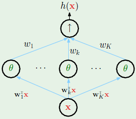
Choosing $\gamma$

The final parameter to choose was the width of the Gaussian curve $\gamma$. This is now treated as a genuine parameter to be learned using an iterative approach using an algorithm known as the Expectation Maximization (EM) algorithm, which is used for solving the mixture of Gaussians. The algorithm is as follows:

1. Fix $\gamma$, solve for $w_1, \dots, w_K$ (using the pseudo-inverse)
2. Fix $w_1, \dots, w_K$, minimize error w.r.t. $\gamma$ (using gradient descent)

With this simple algorithm, we can have different $\gamma_k$ for each center $\center_k$, so that for example one center can “reach out further” than another if it has to.

RBF vs. SVM Kernel

We previously saw the RBF kernel for SVM that implements the following classifier:

We also just saw the straight RBF classifier implementation:

The performance of both models can be observed in the image below. It’s apparent from the straight RBF implementation that $\insample \ne 0$ since some points are misclassified. The SVM implementation clearly tracks the target better, with $\insample = 0$.

RBF Regularization

RBFs can be derived based purely on regularization. Take a 1D function with many data points and we want to inter/extra-polate between the points in order to get the whole function. With regularization there are usually two terms: one two minimize $\insample$ and the regularization term.

The in-sample error minimization term can be defined the squared difference between the hypothesis value and the target value:

A “smoothness” constraint can be added, which is a constraint on the derivatives, by taking the kth-derivative of the hypothesis and squaring it, since we are only interested in the magnitude of it, and integrate it from $-\infty$ to $\infty$. This would be an estimate of the size of the kth-derivative, where if it’s big then it’s bad for smoothness and vice versa. We can then combine the contributions of different derivatives:

These terms can be combined by adding them, but first multiplying the second term by the regularization parameter $\lambda$. We can then minimize the augmented error $\augerror$ where the bigger $\lambda$ is, the more insistent we are on smoothness versus fitting, as we have seen before on the topic of regularization.

If this is solved, we end up with RBFs, which means that with RBFs we are effectively looking for an interpolation, specifically as smooth an interpolation as possible in the sense of the sum of the squares of the derivatives with these coefficients. It isn’t surprising, therefore, that the best interpolation would be Gaussian. This is what gives RBFs credibility as inherently self-regularized.

Three Learning Principles

Occam’s Razor

Occam’s razor is a symbolic principle set by William of Occam, where we have a razor and we keep trimming the explanation to the bare minimum that is still consistent with the data, which happens to be the best possible explanation. More succinctly, it says that:

The simplest model that fits the data is also the most plausible.

Occam’s Razor applied to ML

It’s therefore important to know when a model is considered “simple,” and for this purpose there are two main types of complexity measures: one being the complexity of the hypothesis $h$ (object), the second being the complexity of the hypothesis set $\mathcal H$ (set of objects).

The complexity of $h$ can be measured using minimum description length (MDL) or the order of the polynomial. MDL concerns specifying an object with as few bits as possible, the fewer the bits, the “simpler” the object. For example, for a million-digit number we want to determine the complexity of individual numbers of that length. If we choose the number $2^{1,000,000} - 1$, which is a million digits long, all the number $9$. Despite the fact that this is a very long number, it’s simple because we can simply describe it as $2^{1,000,000} - 1$, which isn’t a very long description. The order of the polynomial as a measure of complexity is straightforward.

The complexity of $\mathcal H$ can be measured using entropy and the VC dimension. The VC dimension produces a number that describes the diversity of the set, which is considered the complexity.

When we think of “simple”, we think in terms of a single object, $h$ in this case. However, proofs use “simple” in terms of $\mathcal H$.

The complexity of an object and a set of objects are related, if not almost identical. For example, using the MDL we take $l$ bits to specify the object $h$, in other words, the complexity of $h$ is $l$ bits. This implies that $h$ is one of $2^l$ elements of a set $\mathcal H$, in other words, one of $2^l$ is the complexity of set $\mathcal H$. Put into words, the link is that something is complex on its own if it’s one of many, whereas something is simple on its own if it’s one of few.

The link holds with respect to real-valued parameters (as opposed to bits), such as a 17th-order polynomial, which is considered complex because it is one of very many, since there are 17 parameters to tune.

There are exceptions. Support vector machines look complex but is one of few, i.e. when we go into an infinite-dimensional space yet only need a few support vectors to represent the separating hyperplane.

Puzzle 1: Football Oracle

You get a letter Monday morning predicting the outcome of Monday night’s game. After we watch the game, we realize the letter was right. The same thing happens next Monday, even with the odds stacked against the team it called. This went on for 5 weeks in a row. On the 6th week, the letter asks you if you want to continue getting predictions for a $50 fee. Should you pay?

We shouldn’t. The guy isn’t sending only to us, but to 32 other people. In the first game, to half of those people he said the home team would lose, and the other half that they would win. The home team lost that first week. The second week, he did the same thing with the half of the recipients for which he sent the correct result. He repeated this process for 5 weeks until there was only one person left for him all “predictions” were correct.

Distribution of Predictions	Result
$\style{color:green}{0000000000000000}\style{color:red}{1111111111111111}$	$0$
$\style{color:green}{00000000}\style{color:red}{11111111}\style{color:gray}{0000000011111111}$	$1$
$\style{color:gray}{00001111}\style{color:green}{0000}\style{color:red}{1111}\style{color:gray}{0000111100001111}$	$0$
$\style{color:gray}{00110011}\style{color:green}{00}\style{color:red}{11}\style{color:gray}{00110011001100110011}$	$1$
$\style{color:gray}{0101010101}\style{color:green}0\style{color:red}1\style{color:gray}{01010101010101010101}$	$1$

We thought that the prediction ability was great since we only saw our letters (and we are the last remaining recipient for which all predictions were “correct”). We figured there was one hypothesis, and it predicted perfectly. The problem is that the hypothesis set is actually very complex, so the prediction value is meaningless, we simply didn’t know since we didn’t see the hypothesis set.

Why is Simpler Better?

Occam’s Razor isn’t making the statement that simpler is more elegant. Instead, Occam’s Razor is making the statement that simpler will have better out-of-sample performance.

The basic argument to back up this claim, which is a formal proof under different idealized conditions, is as follows. There are fewer simpler hypotheses than complex ones, which was captured by the growth function $\growthfunc(N)$. To recap, the growth function took as parameter the size $N$ of the data set and returned the number of different patterns (dichotomies) that the hypothesis set $\mathcal H$ could generate on those $N$ points. Since there are fewer simpler hypotheses, it is less likely to fit a given data set, specifically, $\growthfunc(N)/2^N$. Since it is less likely for fitting to occur, then when it does occur it is more significant.

The only difference between someone believing in the scam in Puzzle #1 and someone having the big picture was the fact that the growth function, from our point of view, was $\growthfunc(N) = 1$—we are only one person, he has one hypothesis, and it was correct, and we gave it a lot of value since that scenario is unlikely to occur. The reality was that the growth function was $\growthfunc(N) = 2^N$, which means it’s certain to happen, so that when it does happen, it’s meaningless.

Meaningless Fit

Suppose two scientists conduct an experiment to determine if conductivity is linear in the temperature. The first scientist is in a hurry so he simply takes two points from the data set and draws a line to connect them. The second scientist took three points and also drew a line. What evidence does the first or second experiment provide for the hypothesis that conductivity is linear in the temperature?

Clearly the experiment that used three points to fit the line provided more evidence than the other. The experiment that used two points provided no evidence at all, because two points can always be connected by a line. This introduces the notion of falsifiability: if your data has no chance of falsifying your assertion, then it doesn’t provide any evidence for the assertion. We have to have a chance to falsify the assertion in order to be able to draw the evidence (axiom of non-falsifiability).

For example, the linear model is too complex for the data set size of $N = 2$ to be able to generalize at all, so there is no evidence. On the other hand, with a data set size of $N = 3$ the assertion could’ve been falsified if one of the three points was not collinear with the other two.

Sampling Bias

Puzzle 2: Presidential Election

In 1948, in the first presidential election after WW2 ended up in a close race between Truman and Dewey. A newspaper ran a phone poll asking people how they voted and concluded that Dewey had won the poll decisively, that is, he won above the error bar. They then printed a newspaper declaring “Dewey Defeats Truman.” However, Truman was the candidate that ended up winning.

This wasn’t $\delta$’s fault, where $\delta$ was the discrepancy between in-sample (poll) and out-of-sample (general population), where we asked ourselves for the probability that this discrepancy is larger than some quantity $\epsilon$ such that the result was flipped:

It was not bad luck, however, because if they had run the poll again with a larger and larger sample size, they would’ve gotten the same result. The problem was that there was a sampling bias in the poll they conducted, and that is that in 1948, phones were expensive, and in that era, rich people favored Dewey more than they favored Truman.

If the data is sampled in a biased way, then learning will produce a similarly biased outcome.

Sampling Bias Principle

This presents a problem of making sure that the data is representative of what we want. For example, in financial forecasting, we may want to predict the market by taking periods of the market where the market was normal. If this model is then tested in the real market which contains non-normal conditions, we will have no idea how the model will perform in those conditions.

Matching the Distributions

The idea is that we have a distribution on the input space in our mind. Remember that VC, Hoeffding’s, etc. made the assumption that we chose the points for training from the same distribution that we picked for testing. One method, in principle, that might resolve this is to make the training set we have be more representative of the target set. This can be done by resampling from the training set by picking data points that better represent the target set, or by scaling the weights of the training points. This could mean that the effective size of the training set decreases, losing some of the independence of the points.

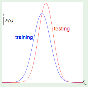
This method doesn’t work if there is a region in the input space where the probability $P = 0$ for training (nothing will be sampled from this region) but $P > 0$ (it’s being tested anyways). This is similar to the people without phones in Puzzle #2, who had $P = 0$ in the sample (they weren’t in the sample) but not in the general population (there were people without phones who voted).

Puzzle 3: Credit Approval

A bank wants to approve credit automatically by going through the historical records of previous applicants who were given credit cards with 3-4 years of credit behavior. The input is the information they provided on the credit application, since this is the data that would be available from a new customer:

data	value
age	23 years
gender	male
annual salary	$30,000
years in residence	1 year
years in job	1 year
current debt	$15,000
…	…

The target is whether or not the person was profitable for the bank. For example, someone flirting with disaster who maxed out but paid the debt was profitable as long as they didn’t default.

The sampling bias lies in the fact that we’re only considering the historical data of customers we approved, since they’re the only ones for whom we have credit behavior data on. When we’re done training, we’ll have a system that applies to a new applicant, and we don’t know beforehand whether or not they’ll be approved or not, because they were never part of our training sample. In this case, sampling bias isn’t entirely terrible, because banks tend to be aggressive in providing credit, since borderline credit users are very profitable.

Data Snooping

The data snooping principle doesn’t forbid us from doing anything, it simply makes us realize that if we use a particular data set—the whole, subset, or something else—to navigate and decide which model, $\lambda$, etc., then when we have an outcome from the learning process and we use the same data set that affected the choice of the learning process, the ability to fairly assess the performance of the outcome has been compromised by the fact that it was chosen according to the data set.

If a data set has affected any step of the learning process, it’s ability to assess the outcome has been compromised.

Data Snooping Principle

This is the most common trap for practitioners. A possible reason is that, when we data snoop, we end up with better performance—or so we think. Data snooping isn’t only looking at the data, in fact there are many ways to fall into the trap.

Looking at the Data

The most common data snooping is “looking at the data.” For example, with non-linear transforms, we use a second-order transform:

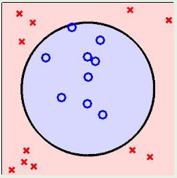
We manage to get $\insample = 0$, so we decide that we fit the problem very well but we don’t like the ratio of parameters-to-data points, with respect to generalization. So we decide that we could’ve done with a simpler transformation:

The problem is that this process of refining the non-linear transformation is essentially a learning algorithm, and we didn’t take into account the fact that we did some of the learning, and thereby forgot to charge the original VC dimension instead of just the final VC dimension of the non-linear transformation we arrived at.

It’s important to realize that the snooping in this example involves the data set $\mathcal D$. The danger of looking at the data set is that we are vulnerable to designing the model or choices in learning according to the idiosyncrasies of the data set, so we are working well on that data set, but we don’t know how we’ll be doing in another independently generated data set from the same distribution, which would be the out-of-sample.

On the other hand, we’re completely allowed—encouraged, ordered—to look at all other information related to the target function and input space, except for the realization of the data set that we’re going to use for training, unless we’re going to charge accordingly. For example, we may ask: how many inputs do we have, what is the range of the inputs, how did we measure the inputs, are they physically correlated, do we know of any properties that we can apply. This is all valid and important for us to zoom-in correctly, since we’re not using the data, and are therefore not subject to overfitting the data. Instead we’re using properties of the target function and input space and therefore improving our chances of picking the correct model. The problem starts when we look at the data set and not charge accordingly.

Puzzle 4: Financial Forecasting

Suppose we want to predict the exchange rate between the US Dollar versus the British Pound. We have 8 years worth of daily trading—about 2,000 data points. Our input-to-output model, where $r$ is the rate, can be expressed as getting the change in rate for the past 20 days, hoping that a particular pattern in the exchange rate will make it more likely that today’s change is positive or negative and by how much:

We normalize the data to zero-mean and unit-variance, we split randomly into a $\trainingset$ of 1,500 points and $\def \testingset {\mathcal D_{\text {test}}}$ and 500 points. The training set is 1,500 days so that for every day (output) we take the previous 20 days as the input. We completely locked away the $\testingset$ until it was time to test, in an effort to avoid data snooping, resulting in:

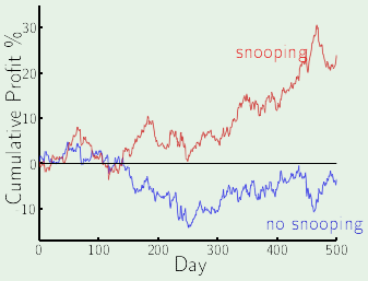
The plot is of the profit that the testing measure represents, which can be seen to be increasing with more and more days that are trained. When we attempt to try this live on the real market, we end up losing a lot money. The fact is that there was actually data snooping in this learning process: when we normalized the data. The problem is that we did this before we separated the data set into $\trainingset$ and $\testingset$, so we took into consideration the mean and variance of the test set.

If we instead split the data first, then only normalized the $\trainingset$ and then took the $\mu$ and $\sigma^2$ that did the normalization for the training set and applied those to the $\testingset$ so that they live in the same range of values and then reran the test, we would’ve gotten the blue line.

To recap, there’s nothing wrong with normalization, as long as the normalization parameters are extracted exclusively from the training set.

Data Set Reuse

If we try one model after another on the same data set, we will eventually “succeed.” The problem is that in doing this, we’re increasing the VC dimension without realizing it, since the final model that we end up using in order to learn is the union of all of the attempted models. Think of the VC dimension of the total learning model.

If you torture the data long enough, it will confess.

This problem could occur not only due to the different models that we have attempted, but also due to what others have attempted. Imagine we decide to try our methods on some data set and we avoid looking at it. We decide to read papers about other people who have used the data set. In the end, we may not have looked at the data ourselves, but we used something that was affected by the data: the papers that others wrote. So that even if we only determined a couple of parameters and yielded great performance, we can’t simply conclude that we have a VC dimension of 2 and 7,000 data points and that we’ll do great out of sample. This is because we don’t only have 2 parameters, but all of the decisions that led up to that model.

The key problem is that we’re matching a particular data set too well; we’re married to the data set, so that a completely new data set generated from the same distribution will look completely foreign to the model we created.

For example, the observation that, in the original data set, whenever a particular pair of points is close, there is always another point on the same line far away—this is clearly an idiosyncrasy of the data set, so that it would be pointless to try to find it in another data set from the same distribution since we may assume that if doesn’t exhibit this same quality, it must be from another distribution. The truth is that the data set is generated from the same distribution, it’s just that we got too used to the data set to the point where we were fitting the noise.

Data Snooping Remedies

There are two remedies to data snooping: avoiding it or accounting for it. Avoiding it naturally requires very strict discipline. Accounting for data snooping concerns keeping track of how much data contamination has occurred on each data set. The most vulnerable part is looking at the data, because it’s very difficult to model ourselves and say what is the hypothesis set that we explored in order to come up with a particular model by looking at the data.

Puzzle 5: Bias via Snooping

We’re testing the long-term performance of a famous strategy in trading called “buy and hold” in stocks. We use 50 years worth of data. We want the test to be as broad as possible so we take all currently traded companies in S&P500. We assume that we strictly followed a buy and hold for all of them. We determine that the model will yield very great profits.

There is a sampling bias because we only looked at the currently traded stocks, which obviously excludes those that were around within the 50-year data span but are no longer traded.

People tend to treat this sampling bias not as sampling bias but as data snooping, because we looked at the future to see which stocks would be traded at that point. We consider it a sampling bias caused by “snooping.”

Epilogue

Map of Machine Learning

Singular value decomposition would treat the Netflix problem as decomposing the canonical ratings matrix into two matrices (user and movie factors). Graphical Models are models for where the target is a joint probability distribution, they try to find computational efficient ways using graph algorithms to determine the joint probability distribution by means of simplifying the graph. Aggregation is when different solutions are combined.

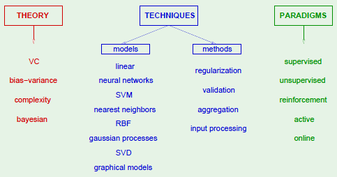
Bayesian Learning

Bayesian learning tries to take a full probabilistic approach to learning. For example, going back to the learning diagram, we can observe that there are many probabilistic components. An inherent probabilistic component is the fact that the target can be noisy, which is why we don’t model the target as a function but rather as a probability distribution. This is apparent in the case of trying to predict heart attacks. Another probability distribution that we had to deal with was the unknown input probability distribution.

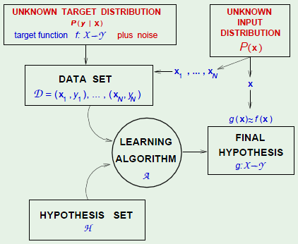
With the Bayesian approach, we want to extend the probabilistic role completely to all components, so that everything is a joint probability distribution. In the case of the heart attack prediction, we were trying to pick the hypothesis by determining the likelihood that that hypothesis would generate the data set in question:

Bayesian approaches instead try to determine the hypothesis by considering the probability that a given hypothesis is the best one given the data:

To compute this probability, we still need one more probability distribution:

The probability $P(\mathcal D \mid h = f)$ can be computed the same way as in logistic regression, and the probability $P(\mathcal D)$ can also be computed by simply integrating out what we don’t want from the joint probability distribution in order to end up with the marginal $P(\mathcal D)$. In fact, since we’re only picking the hypothesis according to the aforementioned criteria, we don’t really care about $P(\mathcal D)$ since it only scales the value up or down, and instead we can only worry about picking the hypothesis that yields the largest numerator.

The quantity that we don’t know is the prior: $P(h = f)$, that is, the probability that the current hypothesis is the target function. It’s called the prior because it’s our belief of the hypothesis set before we got any data. We can modify this value after we get the data to get the posterior: $P(h = f \mid \mathcal D)$, which is more informed based on the data.

Given the prior, we have the full distribution. For example, consider a perceptron $h$ determined by $\weight = w_0, w_1, \dots, w_d$. A possible prior on $\weight$ can take into account the fact that the magnitude of the weights doesn’t matter, so that each weight $w_i$ is independent and uniform over $[-1, 1]$. This determines the prior over $h$, $P(h = f)$. Given $\mathcal D$, we can compute $P(\mathcal D \mid h = f)$. Putting them together we get $P(h = f \mid \mathcal D) \propto P(h = f)P(\mathcal D \mid h = f)$.

This shows that the prior is an assumption. Even the most “neutral” prior for an unknown number $x$ for which we only know that it is between $-1$ and $+1$. It might seem reasonable to want to model this using a uniform probability distribution from $-1$ to $+1$. This seems reasonable because it’s as likely to be any value in that range.

However, consider that using that model, if we were to take a bunch of $x$’s and average them, we’d get something close to $0$. However, in the unknown case, we have no idea what value we’d get from this operation. In fact, we can even say how close it’d be to zero in terms of variance.

In fact, the true equivalent would be the image below, where the probability distribution is a delta function centered on a point $a$ that we don’t know. Choosing to model the situation with the uniform probability distribution results in a huge building based on false premises.

If we actually knew the prior then we could compute the posterior $P(h = f \mid \mathcal D)$ for every hypothesis $h \in \mathcal H$. With this, we could find the most probable hypothesis given the data. In fact, we can derive the expected value of $h$, $\mathbb E(h(\feature))$ for every $\feature$. Further still, we can derive the error bar—the chances that we’re wrong. Simply, we can derive everything in a principled way.

Bayesian learning can be justified in two main cases. The first is when the prior is valid, that is, it is indeed the probability that a particular hypothesis is the target function. The second is when the prior is irrelevant, for example, when we place a prior, when get more and more data sets and we look at the posterior we might realize that the posterior is affected largely by the data set and less by the prior; the prior gets factored out as we get more and more data. In this case, we can think of the prior simply as a computational catalyst.

For example, we might choose to use conjugate priors, where we don’t have to recompute the posterior as an entire function, but instead parameterize it and change the parameters when we get new data points. This is valid when we’re going to be doing it enough that by the time we arrive, it doesn’t matter what we started with.

Aggregation Methods

Aggregation is a method that applies to all models, which combines different solutions $h_1, h_2, \dots, h_T$ that were trained on $\mathcal D$. In the image below, every node corresponds to a resultant system $h_i$ that each person trained.

For example, when trying to detect a face with computer vision, we can instead detect components related to a face, such as an eye, nose, are the positions of these relative to each other, etc. If we were to try to determine whether or not a face was detected from just one of these features, the error would be large. However, if these are combined correctly, we might perform better. This is important in computer vision because we want to perform at or near real-time, so it helps to base the decision on simple computations.

If the problem is a regression, then we can combine the results by simply taking an average. If the problem is a classification, then we can take a vote.

Aggregation is also known as ensemble learning and boosting.

This is different from performing 2-layer learning. For example, in a 2-layer model such as a neural network with one hidden layer, all units learn jointly. In the case of the neural network, each of the nodes are updated jointly via back-propagation. A single node isn’t trying to replicate the function, it’s just trying to contribute positively to the function:

In the case of aggregation, the units learn independently—as if they were the only unit. In the image below, each node is trying to replicate the function individually. Their outputs are then combined to get the output:

Before the Fact

Aggregation before the fact creates the solutions with a view to the fact that they will be combined, such that they will “blend well” together. An example of this is bagging, where we’re given the data set and we resample it so that every solution uses a different bootstrap sample, in order to introduce some independence.

In fact, instead leaving the decorrelation to chance, we can enforce it. We can build each hypothesis by making sure that what it covers is different from what other hypotheses cover. This is done by creating each of the hypotheses $h_1, \dots, h_t, \dots$ sequentially, making each hypothesis $h_t$ decorrelated with previous hypotheses. That is, after the third hypothesis for example, we consider what the best fourth hypothesis would be to add to the mix such that it is sufficiently different from the previous other three. This is accomplished by analyzing how the previous three performed, and based on that performance, providing a data set to the fourth hypothesis so that it develops something fairly independent from the previous three.

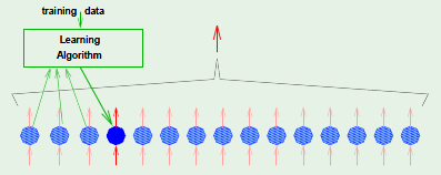
For example, consider that the hypothesis functions that exist so far, combined, can correctly classify 60% of the data points in the set. In order to make the new hypothesis fairly independent from the existing ones, we can emphasize those points on which we performed poorly by giving them larger weights and conversely deemphasize those we got right, such that it looks like 50-50 so that the weighted error is 50%. If we take this distribution and learn on it with the new hypothesis and do better than 50%, then the new hypothesis is adding value to what we had before.

In effect, we choose the weight of $h_t$ based on $\insample(h_t)$. The most famous algorithm that specifies this behavior is adaptive boosting AKA AdaBoost.

After the Fact

Aggregation after the fact combines existing solutions. This is what happened when the Netflix teams merged, “blending.” For regression problems we might have solutions $h_1, h_2, \dots, h_T$, and we might combine the solutions using some coefficients $\alpha$ such that:

To determine the optimal $\alpha$ coefficients, we can minimize the error on a separate “aggregation data set.” The pseudo-inverse can be used for this purpose. It’s important to emphasize that we should use a clean set for the aggregation data set. When this is done, some coefficients may come out negative, but this doesn’t necessarily mean that the solution is bad and is being rid of. It could be that the solution is particularly correlated with another, and so the system is trying to combine them in order to get the signal without the noise.

In that case, how can we determine the most valuable hypothesis in the blend? This can be determined by determining the performance with and without a particular hypothesis, where the difference between these two values corresponds to the contribution of that hypothesis to the blend.

Resources

• Cambridge Information Theory
• Mathematical Monk
• Hugo Larochelle
• Harvard CS 109 — Data Science
• Neural Networks and Deep Learning
• University of Washington Machine Learning by Pedro Domingos
• Neural Networks
• Probabilistic Graphical Models
• Computational Methods for Data Analysis
• Computational Neuroscience
• Mathematical Methods for Quantitative Finance
• UC Berkeley CS 188
• Harvard CS 281 — Advanced Machine Learning
• Recommender Systems
• Introduction to Data Science
• Metacademy
• Probabilistic Programming & Bayesian Methods for Hackers
• Basics of Machine Learning
• Quoc Le’s Lectures on Deep Learning

---

1. How is the gradient derived here? — Math.StackExchange ↩︎